Reflective calculi

This is mostly for my own benefit.

We start with some term-generating functor parametric in a set of ground terms and a set of names .

Now specialize to a single ground term:

Now mod out by structural equivalence:

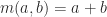
Let be a set of names and let M be the set of name-equivalence classes (where is yet to be defined—it’s part of the theory of names in which we’re still parametric).

Prequoting and predereference are an algebra and coalgebra of , respectively:

such that

Real quoting and dereference have to use , defined below.

Define . Does ? I think so; assuming it does, define

so name equivalence is structural equivalence; equivalence of prequoted predereferences is automatic by the definition above.

The fixed point gives us an isomorphism

We can define , because undecidability doesn’t come into play until we add operational semantics. It’s decidable whether two terms are structurally equivalent. Thus

is the identity, satisfying the condition, and

is the identity, which we get for free.

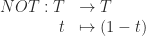
When we mod out by operational semantics (following the traditional approach rather than the 2-categorical one needed for pi calculus):

we have the quotient map

and a map

that picks a representative from the equivalence class.

It’s undecidable whether two terms are in the same operational equivalence class, so may not halt. However, it’s true by construction that

is the identity.

We can extend prequoting and predereference to quoting and dereference on by

and then

which is what we want for quoting and dereference. The other way around involves undecidability.

Monads without category theory, redux

I intended the last version of this post to be a simple one-off, but people cared too much. A fire-breathing Haskellite said that jQuery must never be used as an example of a monad because it’s (gasp) not even functional! And someone else didn’t understand JavaScript well enough to read my code snippets. So here’s another attempt that acknowledges the cultural divide between functional and imperative programmers and tries to explain everything in English as well as in source code.

Monads are a design pattern that is most useful to functional programmers because their languages prefer to implement features as libraries rather than as syntax. In Haskell there are monads for input / output, side-effects and exceptions, with special syntax for using these to do imperative-style programming. Imperative programmers look at that and laugh: “Why go through all that effort? Just use an imperative language to start with.” Functional programmers also tend to write programs as—surprise!—applying the composite of a bunch of functions to some data. The basic operation for a monad is really just composition in a different guise, so functional programmers find this comforting. Functional programmers are also more likely to use “continuations”, which are something like extra-powerful exceptions that only work well when there is no global state; there’s a monad for making them easier to work with.

There are, however, some uses for monads that even imperative programmers find useful. Collections like sets and lists (with or without parentheses), parsers, promises, and membranes are a few examples, which I’ll explain below.

Collections

Many collection types support the following three operations:

1. Map a function over the elements of the collection.
2. Flatten a collection of collections into a collection.
3. Create a collection from a single element.

A monad is a class that provides a generalized version of these three operations. When I say “generalized”, I mean that they satisfy some of the same rules that the collections’ operations satisfy in much the same way that multiplication of real numbers is associative and commutative just like addition of real numbers.

The way monads are usually used is by mapping a function and then flattening. If we have a function f that takes an element and returns a list, then we can say myList.map(f).flatten() and get a new list.

Parsers

A parser is an object with a list of tokens that have already been parsed and the remainder of the object (usually a string) to be parsed.

var Parser = function (obj, tokens) {
  this.obj = obj;
  // If tokens are not provided, use the empty list.
  this.tokens = tokens || [];
};

It has three operations like the collections above.

1. Mapping a function over a parser applies the function to the contained obj.

   Parser.prototype.map = function (f) {
     return new Parser(f(this.obj), this.tokens);
   };
   

2. Flattening a parser of parsers concatenates the list of tokens.

   Parser.prototype.flatten = function () {
     return new Parser(this.obj.obj, this.obj.tokens.concat(this.tokens));
   };
   

   The definition above means that

   new Parser(new Parser(x, tokens1), tokens2).flatten()
   is equivalent to
   new Parser(x, tokens1.concat(tokens2)).

3. We can create a parser from an element x: new Parser(x).

If we have a function f that takes a string, either parses out some tokens or throws an exception, and returns a parser with the tokens and the remainder of the string, then we can say

myParser.map(f).flatten()

and get a new parser. In what follows, I create a parser with the string “Hi there” and then expect a word, then some whitespace, then another word.

var makeMatcher = function (re) {
  return function (s) {
    var m = s.match(re);
    if (!m) { throw new Error('Expected to match ' + re); }
    return new Parser(m[2], [m[1]]);
  };
};

var alnum = makeMatcher(/^([a-zA-Z0-9]+)(.*)/);
var whitespace = makeMatcher(/^(s+)(.*)/);

new Parser('Hi there')
    .map(alnum).flatten()
    .map(whitespace).flatten()
    .map(alnum).flatten(); 
// is equivalent to new Parser('', ['Hi', ' ', 'there']);

Promises

A promise is an object that represents the result of a computation that hasn’t finished yet; for example, if you send off a request over the network for a webpage, the promise would represent the text of the page. When the network transaction completes, the promise “resolves” and code that was waiting on the result gets executed.

1. Mapping a function f over a promise for x results in a promise for f(x).
2. When a promise represents remote data, a promise for a promise is still just remote data, so the two layers can be combined; see promise pipelining.
3. We can create a resolved promise for any object that we already have.

If we have a function f that takes a value and returns a promise, then we can say

myPromise.map(f).flatten()

and get a new promise. By stringing together actions like this, we can set up a computation that will execute properly as various network actions complete.

Membranes

An object-capability language is an object-oriented programming language where you can’t get a reference to an object unless you create it or someone calls one of your methods and passes a reference to it. A “membrane” is a design pattern that implements access control.

Say you have a folder object with a bunch of file objects. You want to grant someone temporary access to the folder; if you give them a reference to the folder directly, you can’t force them to forget it, so that won’t work for revokable access. Instead, suppose you create a “proxy” object with a switch that only you control; if the switch is on, the object forwards all of its method calls to the folder and returns the results. If it’s off, it does nothing. Now you can give the person the object and turn it off when their time is up.

The problem with this is that the folder object may return a direct reference to the file objects it contains; the person could lose access to the folder but could retain access to some of the files in it. They would not be able to have access to any new files placed in the folder, but would see updates to the files they retained access to. If that is not your intent, then the proxy object should hide any file references it returns behind similar new proxy objects and wire all the switches together. That way, when you turn off the switch for the folder, all the switches turn off for the files as well.

This design pattern of wrapping object references that come out of a proxy in their own proxies is a membrane.

1. We can map a function f over a membrane for x and get a membrane for f(x).
2. A membrane for a membrane for x can be collapsed into a single membrane that checks both switches.
3. Given any object, we can wrap it in a membrane.

If we have a function f that takes a value and returns a membrane, then we can say

myMembrane.map(f).flatten()

and get a new membrane. By stringing together actions like this, we can set up arbitrary reference graphs, while still preserving the membrane creator’s right to turn off access to his objects.

Conclusion

Monads implement the abstract operations map and flatten, and have an operation for creating a new monad out of any object. If you start with an instance m of a monad and you have a function f that takes an object and returns a monad, then you can say

m.map(f).flatten();

and get a new instance of a monad. You’ll often find scenarios where you repeat that process over and over.

Overloading JavaScript’s dot operator with direct proxies

With the new ECMAScript 6 Proxy object that Firefox has implemented, you can make dot do pretty much anything you want. I made the dot operator in JavaScript behave like Haskell’s bind:

// I'll give a link to the code for lift() later,
// but one thing it does is wrap its input in brackets.
lift(6); // [6]
lift(6)[0]; // 6
lift(6).length; // 1

// lift(6) has no "upto" property
lift(6).upto; // undefined

// But when I define this global function, ...

// Takes an int n, returns an array of ints [0, ..., n-1].
var upto = function (x) {
  var r = [], i;
  for (i = 0; i < x; ++i) {
    r.push(i);
  }
  return r;
};

// ... now the object lift(6) suddenly has this property
lift(6).upto; // [0,1,2,3,4,5]
// and it automagically maps and flattens!
lift(6).upto.upto; // [0,0,1,0,1,2,0,1,2,3,0,1,2,3,4]
lift(6).upto.upto.length; // 15

To be clear, ECMAScript 6 has changed the API for Proxy since Firefox adopted it, but you can implement the new one on top of the old one. Tom van Cutsem has code for that.

I figured this out while working on a contracts library for JavaScript. Using the standard monadic style (e.g. jQuery), I wrote an implementation that doesn’t use proxies; it looked like this:

lift(6)._(upto)._(upto).value; // [0,0,1,0,1,2,0,1,2,3,0,1,2,3,4]

The lift function takes an input, wraps it in brackets, and stores it in the value property of an object. The other property of the object, the underscore method, takes a function as input, maps that over the current value and flattens it, then returns a new object of the same kind with that flattened array as the new value.

The direct proxy API lets us create a “handler” for a target object. The handler contains optional functions to call for all the different things you can do with an object: get or set properties, enumerate keys, freeze the object, and more. If the target is a function, we can also trap when it’s used as a constructor (i.e. new F()) or when it’s invoked.

In the proxy-based implementation, rather than create a wrapper object and set the value property to the target, I created a handler that intercepted only get requests for the target’s properties. If the target has the property already, it returns that; you can see in the example that the length property still works and you can look up individual elements of the array. If the target lacks the property, the handler looks up that property on the window object and does the appropriate map-and-flatten logic.

I’ve explained this in terms of the list monad, but it’s completely general. In the code below, mon is a monad object defined in the category theorist’s style, a monoid object in an endofunctor category, with multiplication and unit. On line 2, it asks for a type to specialize to. On line 9, it maps the named function over the current state, then applies the monad multiplication. On line 15, it applies the monad unit.

var kleisliProxy = function (mon) {
  return function (t) {
    var mont = mon(t);
    function M(mx) {
      return Proxy(mx, {
        get: function (target, name, receiver) {
          if (!(name in mx)) {
            if (!(name in window)) { return undefined; }
            return M(mont['*'](mon(window[name]).t(mx)));
          }
          return mx[name];
        }
      });
    }
    return function (x) { return M(mont[1](x)); };
  };
};

var lift = kleisliProxy(listMon)(int32);
lift(6).upto.upto; // === [0,0,1,0,1,2,0,1,2,3,0,1,2,3,4]

Semantics for the blue calculus

Blue calculus	MonCat		2Hilb	Set (as a one object bicategory)
Types	monoidal categories	manifolds	2 Hilbert spaces	*
Terms with one free variable	monoidal functors	manifolds with boundary	linear functors	sets
Rewrite rules	monoidal natural transformation	manifolds with corners	linear natural transformations	functions
Tensor product		juxtaposition (disjoint union)	tensor product	cartesian product
where is free		formal sum of cobordisms with boundary from to	sum of linear functors	disjoint union

In the MonCat column, is the categorified version of the tensor product of monoids.

Coends

Coends are a categorified version of “summing over repeated indices”. We do that when we’re computing the trace of a matrix and when we’re multiplying two matrices. It’s categorified because we’re summing over a bunch of sets instead of a bunch of numbers.

Let be a small category. The functor assigns

• to each pair of objects the set of morphisms between them, and
• to each pair of morphisms a function that takes a morphism and returns the composite morphism , where

It turns out that given any functor we can make a new category where and are subcategories and is actually the hom functor; some keywords for more information on this are “collages” and “Artin glueing”. So we can also think of as assigning

• to each pair of objects a set of morphisms between them, and
• to each pair of morphisms a function that takes a morphism and returns the composite morphism , where and

We can think of these functors as adjacency matrices, where the two parameters are the row and column, except that instead of counting the number of paths, we’re taking the set of paths. So is kind of like a matrix whose elements are sets, and we want to do something like sum the diagonals.

The coend of is the coequalizer of the diagram

The top set consists of all the pairs where

• the first element is a morphism and
• the second element is a morphism

The bottom set is the set of all the endomorphisms in

The coequalizer of the diagram, the coend of is the bottom set modulo a relation. Starting at the top with a pair the two arrows give the relation

where I’m using the lollipop to mean a morphism from

So this says take all the endomorphisms that can be chopped up into a morphism from going one way and a from going the other, and then set For this to make any sense, it has to identify any two objects related by such a pair. So it’s summing over all the endomorphisms of these equivalence classes.

To get the trace of the hom functor, use in the analysis above and replace the lollipop with a real arrow. If that category is just a group, this is the set of conjugacy classes. If that category is a preorder, then we’re computing the set of isomorphism classes.

The coend is also used when “multiplying matrices”. Let Then the top set consists of triples the bottom set of pairs and the coend is the bottom set modulo

That is, it doesn’t matter if you think of as connected to or to ; the connection is associative, so you can go all the way from to

Notice here how a morphism can turn “inside out”: when and the identities surround a morphism in , it’s the same as being surrounded by morphisms in and ; this is the difference between a trace, where we’re repeating indices on the same matrix, and matrix multiplication, where we’re repeating the column of the first matrix in the row of the second matrix.

Theories and models

The simplest kind of theory is just a set thought of as a set of concepts or Platonic ideals. We typically have some other set thought of as the set of real things that are described by concepts. Then a model is a function For example, we could let = {0, 1}; this is the theory of the number “two”, since it has two elements. Whatever set we choose for , the models of the theory are going to be pairs of elements of . So if = the set of people, models of in are going to be pairs of people (where choosing the same person twice is allowed).

Concepts, however, are usually related to each other, whereas in a set, you can only ask if elements are the same or not. So the way a theory is usually presented is as a category For example let be the category with two objects and two parallel nontrivial morphisms and let be the category Set of sets and functions. A model is a structure-preserving map from the category to Set, i.e. a functor. Each object of gets mapped to a set; here we think of the image of as a set of vertices and the image of as a set of edges. Each morphism of gets mapped to a function; and take an edge and produce the source vertex or target vertex, respectively. The category = Th(Graph) is the theory of a graph, and its models are all graphs.

Usually, our theories have extra structure. Consider the first example of a model, a function between sets. We can add structure to the theory; for example, we can take the set to be the ring of integers Then a model is a structure-preserving function, a homomorphism between and Of course, this means that has to have at least as much structure as We could, for instance, take to be the real numbers under multiplication. Since this ring homomorphism is entirely determined by where we map 1, and we can choose any real number for its image, there would be one model for each real number; each integer would map to for some Another option is to take the integers modulo 4. There are three nonisomorphic models of in . If we map 1 to 0, we get the trivial ring; if we map 1 to 1 or 3, we get integers modulo 4; and if we map 1 to 2, we get integers modulo 2.

Similarly, we can add structure to a category. If we take monoidal categories then we can tensor objects together to get new ones. A model of such a theory is a tensor-product-preserving functor from to See my paper “Physics, Topology, Computation, and Logic: a Rosetta Stone” with John Baez for a thorough exploration of theories that are braided monoidal closed categories and models of these.

An element of the set is a number, while an object of the category Th(Graph) is a set. A theory is a mathematical gadget in which we can talk about theories of one dimension lower. In Java, we say “interface” instead of “theory” and “class” instead of “model”. With Java interfaces we can describe sets of values and functions between them; it is a cartesian closed category whose objects are datatypes and whose morphisms are (roughly) programs. Models of an interface are different classes that implement that interface.

And there’s no reason to stop at categories; we can consider bicategories with structure and structure-preserving functors between these; these higher theories should let us talk about different models of computation. One model would be Turing machines, another lambda calculus, a third would be the Java Virtual Machine, a fourth Pi calculus.

Renormalization and Computation 4

This is the fourth in a series of posts on Yuri Manin’s pair of papers. In the previous posts, I laid out the background; this time I’ll actually get around to his result.

A homomorphism from the Hopf algebra into a target algebra is called a character. The functor that assigns an action to a path, whether classical or quantum, is a character. In the classical case, it’s into the rig and we take an infimum over paths; in the quantum it’s into the rig and we take an integral over paths. Moving from the quantum to the classical case is called Maslov dequantization.

Manin mentions that the runtime of a parallel program is a character akin to the classical action, with the runtime of the composition of two programs being the sum of the respective runtimes, while the runtime of two parallel programs is the maximum of the two. A similar result holds for nearly any cost function. He also points out that computably enumerable reals form a rig He examines Rota-Baxter operators as a way to generalize what “polar part” means and extend the theorems on Hopf algebra renormalization to such rigs.

In the second paper, he looks at my work with Calude as an example of a character. He uses our same argument to show that lots of measures of program behavior have the property that if the measure hasn’t stopped growing after reaching a certain large amount with respect to the program size, then the density of finite values the measure could take decreases like Surprisingly, though he referred to these results as cutoffs, he didn’t actually use them anywhere for doing regularization.

Reading between the lines, he might be suggesting something like approximating the Kolmogorov complexity that he uses later by using a time cutoff, motivated by results from our paper: there’s a constant depending only on the programming language such that if you run the th program steps and it hasn’t stopped, then the density of times near at which it could stop is roughly

Levin suggested using a computable complexity that’s the sum of the program length and the log of the number of time steps; I suppose you could “regularize” the Kolmogorov complexity by adding to the length of the program, renormalize, and then let go to zero, but that’s not something Manin does.

Instead, he proposed two other constructions suitable for renormalization; here’s the simplest. Given a partial computable function define the computably enumerable by if is defined, and 0 otherwise. Now define

When is undefined, which has a pole at When is defined, converges everywhere except Birkhoff decomposition would separate these two cases, though I’m not sure what value would take or what it would mean.

The other construction involves turning into a permutation and inventing a function that has poles when the permutation has fixpoints.

So Manin’s idea of renormalizing the halting problem is to do some uncomputable stuff to get an easy-to-renormalize function and then throw the Birkhoff decomposition at it; since we know the halting problem is undecidable, perhaps the fact that he didn’t come up with a new technique for extracting information about the problem is unsurprising, but after putting in so much effort to understand it, I was left rather disappointed: if you’re going to allow yourself to do uncomputable things, why not just solve the halting problem directly?

I must suppose that his intent was not to tackle this hard problem, but simply to play with the analogy he’d noticed; it’s what I’ve done in other papers. And being forced to learn renormalization was exhilarating! I have a bunch of ideas to follow up; I’ll write them up as I get a chance.

Renormalization and Computation 1

Yuri Manin recently put two papers on the arxiv applying the methods of renormalization to computation and the Halting problem. Grigori Mints invited me to speak on Manin’s results at the weekly Stanford logic seminar because in his second paper, he expands on some of my work.

In these next few posts, I’m going to cover the idea of Feynman diagrams (mostly taken from the lecture notes for the spring 2004 session of John Baez’s Quantum Gravity seminar); next I’ll talk about renormalization (mostly taken from Andrew Blechman’s overview and B. Delamotte’s “hint”); third, I’ll look at the Hopf algebra approach to renormalization (mostly taken from this post by Urs Schreiber on the n-Category Café); and finally I’ll explain how Manin applies this to computation by exploiting the fact that Feynman diagrams and lambda calculus are both examples of symmetric monoidal closed categories (which John Baez and I tried to make easy to understand in our Rosetta stone paper), together with some results on the density of halting times from my paper “Most programs stop quickly or never halt” with Cris Calude. I doubt all of this will make it into the talk, but writing it up will make it clearer for me.

Renormalization is a technique for dealing with the divergent integrals that arise in quantum field theory. The quantum harmonic oscillator is quantum field theory in 0+1 dimensions—it describes what quantum field theory would be like if space consisted of a single point. It doesn’t need renormalization, but I’m going to talk about it first because it introduces the notion of a Feynman diagram.

“Harmonic oscillator” is a fancy name for a rock on a spring. The force exerted by a spring is proportional to how far you stretch it:

The potential energy stored in a stretched spring is the integral of that:

and to make things work out nicely, we’re going to choose The total energy is the sum of the potential and the kinetic energy:

By choosing units so that we get

where is momentum.

Next we quantize, getting a quantum harmonic oscillator, or QHO. We set taking units where Now

If we define a new observable then

We can think of as and write the energy eigenvectors as polynomials in

The creation operator adds a photon to the mix; there’s only one way to do that, so The annihilation operator destroys one of the photons; in the state , there are photons to choose from, so

Schrödinger’s equation says so

This way of representing the state of a QHO is known as the “Fock basis”.

Now suppose that we don’t have the ideal system, that the quadratic potential is only a good local approximation to the real potential . Then we can write the total as where is a function of position and momentum, or equivalently of and and is small.

Now we solve Schrödinger’s equation perturbatively. We know that

and we assume that

so that it makes sense to solve it perturbatively. Define

and

After a little work, we find that

and integrating, we get

We feed this equation back into itself recursively to get

So here we have a sum of a bunch of terms; the th term involves interactions with the potential interspersed with evolving freely between the interactions, and we integrate over all possible times at which those interactions could occur.

Here’s an example Feynman diagram for this simple system, representing the fourth term in the sum above:

The lines represent evolving under the free Hamiltonian , while the dots are interactions with the potential .

As an example, let’s consider and choose so that When acts on a state we get So at each interaction, the system either gains a photon or changes phase and loses a photon.

A particle moving in a quadratic potential in -dimensional space gives the tensor product of QHOs, which is QFT in a space where there are possible harmonics. Quantum electrodynamics (QED) amounts to considering infinitely many QHOs, one for each possible energy-momentum, which forms a continuum. The diagrams for QED start to look more familiar:

The vertices are interactions with the electromagnetic field. The straight lines are electrons and the wiggly ones are photons; between interactions, they propagate under the free Hamiltonian.

Monad for weakly monoidal categories

We’ve got free and forgetful functors Define Given a category the category has

• binary trees with labeled leaves as objects and
• binary trees with labeled leaves together with the natural isomorphisms from the definition of a weakly monoidal category as its morphisms.

The multiplication collapses two layers of trees down to one. The unit gives a one-leaf tree.

An algebra of the monad is a category together with a functor such that and Define

Then the associator should be a morphism

However, it isn’t immediately evident that the associator that comes from does the job, since just applying to gives

for the source instead of

,

which we get by replacing with its definition above. We need an isomorphism

so we can define Now we use the equations an algebra has to satisfy to derive this isomorphism. Since the following two objects are equal:

Therefore, the isomorphism we wanted is simply equality and It also means that satisfies the pentagon equation.

A similar derivation works for the unitors and the triangle equation.

A morphism of algebras is a functor such that Now

and

so we have the coherence laws for a strict monoidal functor.

Also,

so it preserves the associator as well. The unitors follow in the same way, so morphisms of these algebras are strict monoidal functors that preserve the associator and unitors.

Functors and monads

In many languages you have type constructors; given a type A and a type constructor Lift, you get a new type Lift<A>. A functor is a type constructor together with a function

   lift: (A -> B) -> (Lift<A> -> Lift<B>)

that preserves composition and identities. If h is the composition of two other functions g and f

   h (a) = g (f (a)),

then lift (h) is the composition of lift (g) and lift (f)

   lift (h) (la) = lift (g) (lift (f) (la)),

where the variable la has the type Lift<A>. Similarly, if h is the identity function on variables of type A

   h (a: A) = a,

then lift (h) will be the identity on variables of type Lift<A>

   lift (h) (la) = la.

Examples:

• Multiplication
  Lift<> adjoins an extra integer to any type:

     Lift<A> = Pair<A, int>

  The function lift() pairs up f with the identity function on integers:

     lift (f) = (f, id)

• Concatenation
  Lift<> adjoins an extra string to any type:

     Lift<A> = Pair<A, string>

  The function lift() pairs up f with the identity function on strings:

     lift (f) = (f, id)

• Composition
  Let Env be a type representing the possible states of the environment and

     Effect = Env -> Env

  Also, we’ll be explicit in the type of the identity function

     id<A>: A -> A
     id<A> (a) = a,

  so one possible Effect is id<Env>, the “trivial side-effect”.

  Then Lift<> adjoins an extra side-effect to any type:

     Lift<A> = Pair<A, Effect>

  The function lift() pairs up f with the identity on side-effects:

     lift (f) = (f, id<Effect>)

• Lists
  The previous three examples used the Pair type constructor to adjoin an extra value. This functor is slightly different. Here, Lift<> takes any type A to a list of A‘s:

     Lift<A> = List<A>

  The function lift() is the function map():

     lift = map

• Double negation, or the continuation passing transform
  In a nice type system, there’s the Unit type, with a single value, and there’s also the Empty type, with no values (it’s “uninhabited”). The only function of type X -> Empty is the identity function id<Empty>. This means that we can think of types as propositions, where a proposition is true if it’s possible to construct a value of that type. We interpret the arrow as implication, and negation can be defined as “arrowing into Empty“: let F = Empty and T = F -> F. Then T -> F = F (since T -> F is uninhabited) and T is inhabited since we can construct the identity function of type F -> F. Functions correspond to constructive proofs. “Negation” of a proof is changing it into its contrapositive form:

    If A then B => If NOT B then NOT A.

  Double negation is doing the contrapositive twice:

    IF A then B => If NOT NOT A then NOT NOT B.

  Here, Lift<> is double negation:

     Lift<A> = (A -> F) -> F.

  The function lift takes a proof to its double contrapositive:

     lift: (A -> B)   ->   ((A -> F) -> F) -> ((B -> F) -> F)
     lift  (f) (k1) (k2) = k1 (lambda (a) { k2 (f (a)) })

Monads

A monad is a functor together with two functions

   m: Lift<Lift<A>> -> Lift<A>
   e: A -> Lift<A>

satisfying some conditions I’ll get to in a minute.

Examples:

• Multiplication
  If you adjoin two integers, m() multiplies them to get a single integer:

     m: Pair<Pair<A, int>, int> -> Pair<A, int>
     m  (a, i, j)               =  (a, i * j).

  The function e() adjoins the multiplicative identity, or “unit”:

     e: A   -> Pair<A, int>
     e  (a) = (a, 1)

• Concatenation
  If you adjoin two strings, m() concatenates them to get a single string:

     m: Pair<Pair<A, string>, string> -> Pair<A, string>
     m  (a, s, t)                     =  (a, s + t).

  The function e() adjoins the identity for concatenation, the empty string:

     e: A   -> Pair<A, string>
     e  (a) = (a, "")

• Composition
  If you adjoin two side-effects, m() composes them to get a single effect:

     m: Pair<Pair<A, Effect>, Effect> -> Pair<A, Effect>
     m  (a, s, t)                     =  (a, t o s),

  where

     (t o s) (x) = t (s (x)).

  The function e() adjoins the identity for composition, the identity function on Env:

     e: A   -> Pair<A, Effect>
     e  (a) = (a, id<Env>)

• Lists
  If you have two layers of lists, m() flattens them to get a single layer:

     m: List<List<A>> -> List<A>
     m = flatten

  The function e() makes any element of A into a singleton list:

     e: A -> List<A>
     e (a) = [a]

• Double negation, or the continuation passing transform
  If you have a quadruple negation, m() reduces it to a double negation:

     m: ((((A -> F) -> F) -> F) -> F)   ->  ((A -> F) -> F)
     m (k1) (k2) = k1 (lambda (k3) { k3 (k2) })

  The function e() is just reverse application:

     e: A -> (A -> F) -> F
     e (a) (k) = k (a)

The conditions that e and m have to satisfy are that m is associative and e is a left and right unit for m. In other words, assume we have

   llla: Lift<Lift<Lift<A>>>
   la: Lift<A>

Then

   m (lift (m) (llla))  =  m (m (llla))

and

   m (e (la))  =  m (lift (e) (la))  =  la

Examples:

• Multiplication:
  There are two different ways we can use lifting with these two extra functions e() and m(). The first is applying lift() to them. When we apply lift to m(), it acts on three integers instead of two; but because

     lift (m) = (m, id),

  it ignores the third integer:

     lift (m) (a, i, j, k) = (a, i * j, k).

  Similarly, lifting e() will adjoin the multiplicative unit, but will leave the last integer alone:

     lift (e) = (e, id)
     lift (e) (a, i) = (a, 1, i)

  The other way to use lifting with m() and e() is to apply Lift<> to their input types. This specifies A as Pair<A', int>, so the first integer gets ignored:

     m (a, i, j, k) = (a, i, j * k)
     e (a, i) = (a, i, 1)

  Now when we apply m() to all of these, we get the associativity and unit laws. For associativity we get

     m (lift (m) (a, i, j, k)) = m(a, i * j, k) = (a, i * j * k)
     m (m (a, i, j, k)) = m(a, i, j * k) = (a, i * j * k)

  and for unit, we get

     m (lift (e) (a, i)) = m (a, 1, i) = (a, 1 * i) = (a, i)
     m (e (a, i)) = m (a, i, 1) = (a, i * 1) = (a, i)

• Concatenation
  There are two different ways we can use lifting with these two extra functions e() and m(). The first is applying lift() to them. When we apply lift to m(), it acts on three strings instead of two; but because

     lift (m) = (m, id),

  it ignores the third string:

     lift (m) (a, s, t, u) = (a, s + t, u).

  Similarly, lifting e() will adjoin the empty string, but will leave the last string alone:

     lift (e) = (e, id)
     lift (e) (a, s) = (a, "", s)

  The other way to use lifting with m() and e() is to apply Lift<> to their input types. This specifies A as Pair<A', string>, so the first string gets ignored:

     m (a, s, t, u) = (a, s, t + u)
     e (a, s) = (a, s, 1)

  Now when we apply m() to all of these, we get the associativity and unit laws. For associativity we get

     m (lift (m) (a, s, t, u)) = m(a, s + t, u) = (a, s + t + u)
     m (m (a, s, t, u)) = m(a, s, t + u) = (a, s + t + u)

  and for unit, you get

     m (lift (e) (a, s)) = m (a, "", s) = (a, "" + s) = (a, s)
     m (e (a, s)) = m (a, s, "") = (a, s + "") = (a, s)

• Composition
  There are two different ways we can use lifting with these two extra functions e() and m(). The first is applying lift() to them. When we apply lift to m(), it acts on three effects instead of two; but because

     lift (m) = (m, id<Effect>),

  it ignores the third effect:

     lift (m) (a, s, t, u) = (a, t o s, u).

  Similarly, lifting e() will adjoin the identity function, but will leave the last string alone:

     lift (e) = (e, id<Effect>)
     lift (e) (a, s) = (a, id<Env>, s)

  The other way to use lifting with m() and e() is to apply Lift<> to their input types. This specifies A as Pair<A', Effect>, so the first effect gets ignored:

     m (a, s, t, u) = (a, s, u o t)
     e (a, s) = (a, s, id<Env>)

  Now when we apply m() to all of these, we get the associativity and unit laws. For associativity we get

     m (lift (m) (a, s, t, u)) = m(a, t o s, u) = (a, u o t o s)
     m (m (a, s, t, u)) = m(a, s, u o t) = (a, u o t o s)

  and for unit, you get

     m (lift (e) (a, s)) = m (a, id<Env>, s) = (a, s o id<Env>) = (a, s)
     m (e (a, s)) = m (a, s, id<Env>) = (a, id<Env> o s) = (a, s)

• Lists
  There are two different ways we can use lifting with these two extra functions e() and m(). The first is applying lift() to them. When we apply lift to m(), it acts on three layers instead of two; but because

     lift (m) = map (m),

  it ignores the third (outermost) layer:

       lift (m) ([[[a, b, c], [], [d, e]], [[]], [[x], [y, z]]])
     = [[a, b, c, d, e], [], [x, y, z]]

  Similarly, lifting e() will make singletons, but will leave the outermost layer alone:

     lift (e) ([a, b, c]) = [[a], [b], [c]]

  The other way to use lifting with m() and e() is to apply Lift<> to their input types. This specifies A as List<A'>, so the *innermost* layer gets ignored:

       m ([[[a, b, c], [], [d, e]], [[]], [[x], [y, z]]])
     = [[a, b, c], [], [d, e], [], [x], [y, z]]
  
     e ([a, b, c]) = [[a, b, c]]

  Now when we apply m() to all of these, we get the associativity and unit laws. For associativity we get

       m (lift (m) ([[[a, b, c], [], [d, e]], [[]], [[x], [y, z]]]))
     = m([[a, b, c, d, e], [], [x, y, z]])
     = [a, b, c, d, e, x, y, z]
  
       m (m ([[[a, b, c], [], [d, e]], [[]], [[x], [y, z]]]))
     = m([[a, b, c], [], [d, e], [], [x], [y, z]])
     = [a, b, c, d, e, x, y, z]

  and for unit, we get

     m (lift (e) ([a, b, c])) = m ([[a], [b], [c]]) = [a, b, c]
     m (e ([a, b, c])) = m ([[a], [b], [c]]) = [a, b, c]

Monads in Haskell style, or “Kleisli arrows”

Given a monad (Lift, lift, m, e), a Kleisli arrow is a function

   f: A -> Lift<B>,

so the e() function in a monad is already a Kleisli arrow. Given

   g: B -> Lift<C>

we can form a new Kleisli arrow

   (g >>= f): A -> Lift<C>
   (g >>= f) (a) = m (lift (g) (f (a))).

The operation >>= is called “bind” by the Haskell crowd. You can think of it as composition for Kleisli arrows; it’s associative, and e() is the identity for bind. e() is called “return” in that context. Sometimes code is less complicated with bind and return instead of m and e.

If we have a function f: A -> B, we can turn it into a Kleisli arrow by precomposing with e():

   (e o f): A -> Lift<B>
   (e o f) (a) = e (f (a)) = return (f (a)).

Example:

• Double negation, or the continuation passing style transform
  We’re going to (1) show that the CPS transform of a function takes a continuation and applies that to the result of the function.  We’ll also (2) show that for two functions r, s,

       CPS (s o r)    =    CPS (s) >>= CPS (r),

  (1) To change a function f: A -> B into a Kleisli arrow (i.e. continuized function) CPS (f): A -> (B -> X) -> X, we just compose with e—or in the language of Haskell, we return the result:

       CPS (f) (a) (k)
     = return (f (a)) (k)
     = (e o f) (a) (k)
     = e (f (a)) (k)
     = k (f (a))

  (2) Given two Kleisli arrows

     f: A -> (B -> F) -> F

  and

     g: B -> (C -> F) -> F,

  we can bind them:

       (g >>= f) (a) (k)
     = m (lift (g) (f (a))) (k)                                // defn of bind
     = lift (g) (f (a)) (lambda (k3) { k3 (k) })               // defn of m
     = f (a) (lambda (b) { (lambda (k3) { k3 (k) }) (g (b)) }) // defn of lift
     = f (a) (lambda (b) { g (b) (k) }),                       // application

  which is just what we wanted.

  In particular, if f and g are really just continuized functions

     f = (e o r)
     g = (e o s)

  then

       (g >>= f) (a) (k)
     = f (a) (lambda (b) { g (b) (k) })             // by above
     = (e o r) (a) (lambda (b) { (e o s) (b) (k) }) // defn of f and g
     = (e o r) (a) (lambda (b) { k (s (b)) })       // defn of e
     = (e o r) (a) (k o s)                          // defn of composition
     = (k o s) (r (a))                              // defn of e
     = k (s (r (a)))                                // defn of composition
     = (e o (s o r)) (a) (k)                        // defn of e
     = CPS (s o r) (a) (k)                          // defn of CPS

  so

     CPS (s) >>= CPS (r)    =    CPS (s o r).

My talk at Perimeter Institute

I spent last week at the Perimeter Institute, a Canadian institute founded by Mike Lazaridis (CEO of RIM, maker of the BlackBerry) that sponsors research in cosmology, particle physics, quantum foundations, quantum gravity, quantum information theory, and superstring theory. The conference, Categories, Quanta, Concepts, was organized by Bob Coecke and Andreas Döring. There were lots of great talks, all of which can be found online, and lots of good discussion and presentations, which unfortunately can’t. (But see Jeff Morton’s comments.) My talk was on the Rosetta Stone paper I co-authored with Dr. Baez.

Syntactic string diagrams

I hit on the idea of making lambda a node in a string diagram, where its inputs are an antivariable and a term in which the variable is free, and its output is the same term, but in which the variable is bound.  This allows a string diagram notation for lambda calculus that is much closer to the syntactical description than the stuff in our Rosetta Stone paper. Doing it this way makes it easy to also do pi calculus and blue calculus.

There are two types, V (for variable) and T (for term). I’ve done untyped lambda calculus, but it’s straightforward to add subscripts to the types V and T to do typed lambda calculus.

There are six function symbols:

• Lambda takes an antivariable and a term that may use the corresponding variable.
• This turns an antivariable “x” introduced by lambda into the term “x”.
• (Application) This takes and and produces .
• 
• 
• These two mean we can duplicate and delete terms.

The rule is the real meat of the computation. The “P” is an arbitrary subdiagram. The effect is replacing the “A” application node with the “P” subdiagram, modulo some wiring.

I label the upwards arrows out of lambdas with a variable name in parentheses; this is just to assist in matching up the syntactical representation with the string diagram.

In the example, I surround part of the diagram with a dashed line; this is the part to which the rule applies. Within that, I surround part with a dash-dot line; this is the subdiagram P in the rule.

When I do blue calculus this way, there are a few more function symbols and the relations aren’t confluent, but the flavor is very much the same.

String diagrams for untyped lambda calculus

An example calculation

I finally understand the state transformer monad!

It’s the monad arising from the currying adjunction between and   attaches an environment to :

This is the type of a function that takes a state of type and outputs a result of type and a new state of type . So is the ability to depend on state and is the ability to change the state.

The natural transformation is evaluation:

takes a function and an input point and evaluates the function at that point.  So we get

by evaluating the in the middle, while the unit

is just the curried identity on pairs:

Reading list

http://www.haskell.org/haskellwiki/Category_theory#Categorical_programming

http://www.cl.cam.ac.uk/~mpf23/

Yoneda embedding as contrapositive and call-cc as double negation

Consider the problem of how to represent negation of a proposition when we only have implication and falsehood:

Since is true and is false, this does what we want.

The contrapositive says has the same truth value as Using only implication, the contrapositive of is

What if we don’t even have falsehood? Well, we can pick any proposition to represent falsehood and form

The Yoneda embedding takes a category and produces a category :

This embedding is better known among computer scientists as the continuation passing style transformation.

In a symmetric monoidal closed category, like lambda calculus, we can move everything “inside:” every morphism has an internal version The internal Yoneda embedding of is

Here is the “unit” type; notice how the target type is isomorphic under the Curry-Howard isomorphism to the contrapositive. This is a term that maps a continuation and a value to

To get double negation, first do the Yoneda embedding on the identity to get

then uncurry, braid, and recurry to get

or, internally,

This takes a value to a function value

Call-with-current-continuation expects a term that has been converted to CPS style as above, and then hands it the remainder of the computation in

The category GraphUp

The category GraphUp of graphs and Granovetter update rules has

• directed finite graphs as objects
• morphisms generated by Granovetter rules, i.e. the following five operations:
  • add a new node. (creation, refcount=0)
  • given a node add a new node and an edge (creation, refcount=1)
  • given edges and add an edge (introduction, ++refcount)
  • remove an edge. (deletion, --refcount)
  • remove a node and all its outgoing edges if it has no incoming edges. (garbage collection)

It’s a monoidal category where the tensor product is disjoint union. Also, since two disjoint graphs can never become connected, they remain disjoint.

Programs in a capability-secure language get interpreted in GraphUp. A program’s state graph consists of nodes, representing the states of the system, and directed edges, representing the system’s transitions between states upon receiving input. A functor from a program state graph to GraphUp assigns an object reference graph as state to each node and an update generated by Granovetter rules to each edge.

Haskell monads for the category theorist

A monad in Haskell is about composing almost-compatible morphisms. Typically you’ve got some morphism and then you think of a reason that you’d rather have where is a functor. In Haskell, though, you don’t define functors right out: you define type constructors, which are like the map of objects in a functor. You have to define the map of morphisms separately.

To define the map of morphisms, we have to define (aka ) and . We define to be the category-theorist’s unit composed with the input. Applying to gives

To compose “half-functored” morphisms like we define like this: given an input and a morphism like bind produces

So a “monad” in Haskell is always the monad for categories, except the lists are of bindable half-functored morphisms like rather than lists of composable morphisms.

A side-effect monad has where is the data type for the environment on which the morphism is to act. The IO monad is a specific instance of a side-effect monad with the environment being the keyboard queue, disk drive, network, etc.

Another piece of the stone

A few days ago, I thought that I had understood pi calculus in terms of category theory, and I did, in a way.

calculus model in Set type set of values term function (deterministic outcome) rewrite rule identity functional

calculus model in Set process set of states reduction rule state update rule (deterministic outcome)

To make lambda calculus into a category, we mod out by the rewrite rules and consider equivalence classes of terms instead of actual terms. A model of this category (i.e. a functor from the category to Set) picks out a set of values for each datatype and a function for each program. Given a value from the input set, we get a single value from the output set.

Similarly, a model of the pi calculus assigns to each process a set of states and to each reduction rule a function that updates the state. A morphism in this way of thinking is a certain number of reductions to perform. The reductions are deterministic in the sense that we can model “A or B” as Given an object’s state at a certain point, we can tell what set of states it can be in after the system reduces n messages.

However, what we really want is to know the set of states it can be in after all the messages have been processed: what is its normal form? This is far more like the rewrite rules in lambda calculus. It suggests that we should be treating the reduction rules like 2-morphisms instead of 1-morphisms. There’s one important difference from lambda calculus, however: the 2-morphisms of pi calculus are not confluent! It matters very much in which order they are evaluated. Thus processes can’t map to anything but trivial functions.

It looks like a better fit for models of the pi calculus is Rel, the category of sets and relations. A morphism in Rel can relate a single input state to multiple output states. This suggests we have a single object * in the pi calculus that gets mapped to a set of possible states for the system, while each process gets mapped to a relation that encodes all its possible reductions.

I’m rather embarrassed that it took me so long to notice this, since my advisor has been talking about replacing Set by Rel for years.

category	lambda calculus	pi calculus
objects	types	only one type *, a system of processes
a morphism	an equivalence class of terms	a structural congruence class of processes
dinatural transformation from the constant functor (mapping to the terminal set and its identity) to a functor generated by hom, products, projections, and exponentials (if they’re there)	combinator: template for programs mapping between isomorphic types (usually)	since there’s only one type, this is trivial
Model of the category in Rel	(usually taken in Set, a subcategory of Rel) a set of values for each data type and a function for each morphism between them	* maps to a set S of states for the system, and each process gets mapped to a relation that relates each element of S to its possible reductions in S

The Yoda embedding

Continuation passing as a reflection

We can write any expression like as a full binary tree where the nodes denote evaluation of the left child at the right, and the leaves are values:

Figure 1:

[In the caption of figure 1, the expression is slightly different; when using trees, it’s more convenient to curry all the functions—that is, replace every comma “,” by back-to-back parens: “)(” .]

The continuation passing transform (Yoneda embedding) first reflects the tree across the vertical axis and then replaces the root and all the left children with their continuized form—a value gets replaced with a function value

Figure 2:

What does this evaluate to? Well,

As we hoped, it’s the continuization (Yoneda embedding) of the original expression. Iterating, we get

Figure 3:

At this point, we get an enormous simplification: we can get rid of overlines whenever the left and right branch both have them. For instance,

Actually working out the whole expression would mean lots of epicycular reductions like this one, but taking the shortcut, we just get rid of all the lines except at the root. That means that we end up with

for our final expression.

However, if this expression is just part of a larger one—if what we’re calling the “root” is really the child of some other node—then the cancellation of lines on siblings applies to our “root” and its sibling, and we really do get back to where we started!

A piece of the Rosetta stone

category	lambda calculus	pi calculus	Turing machine
objects	types	structural congruence classes of processes	where is the natural numbers and is all binary sequences with finitely many ones.
a morphism	an equivalence class of terms	a specific reduction from one process state to the next	a specific transition from one state and position of the machine to the next
dinatural transformation from the constant functor (mapping to the terminal set and its identity) to a functor generated by hom, products, projections, and exponentials (if they’re there)	combinator	reduction rule (covers all reductions of a particular form)	tape-head update rule (covers all transitions with the current cell and state in common)
products	product types	parallel processes	multiple tapes
internal hom	exponential types	all types are exponentials?	?
Model of the category in Set	A set of values for each data type and a function for each morphism between them	A set of states for each process and a single evolution function out of each set.	?

This won’t be appearing in our Rosetta stone paper, but I wanted to write it down. What flavor of logic corresponds to the pi calculus? To the Turing machine?

The continuation passing transform and the Yoneda embedding

They’re the same thing! Why doesn’t anyone ever say so?

Assume A and B are types; the continuation passing transform takes a function (here I’m using C++ notation)

B f(A a);

and produces a function

 CPT_f( (*k)(B), A a) {
  return k(f(a));
}

where X is any type. In CPT_f, instead of returning the value f(a) directly, it reads in a continuation function k and “passes” the result to it. Many compilers use this transform to optimize the memory usage of recursive functions; continuations are also used for exception handling, backtracking, coroutines, and even show up in English.

The Yoneda embedding takes a category and produces a category :

We get the transformation above by uncurrying to get

In Java, a (cartesian closed) category is an interface C with a bunch of internal interfaces and methods mapping between them. A functor is written

class F implements C.

Then each internal interface C.A gets instantiated as a set F.A of values and each method C.f() becomes instantiated as a function F.f() between the sets.

The continuation passing transform can be seen as a parameterized functor . We’d write

class CPT<X> implements C.

Then each internal interface C.A gets instantiated as a set CPT.A of methods mapping from C.A to X—i.e. continuations that accept an input of type C.A—and each method C.f maps to the continuized function CPT.f described above.

Then the Yoneda lemma says that for every model of —that is, for every class F implementing the interface C—there’s a natural isomorphism between the set and the set of natural transformations

A natural transformation between and is a way to cast the class F to the class CPT<X> such that for any method of C, you can either

• invoke its implementation directly (as a method of F) and then continuize the result (using the type cast), or
• continuize first (using the type cast) and then invoke the continuized function (as a method of CPT<X>) on the result

and you’ll get the same answer. Because it’s a natural isomorphism, the cast has an inverse.

The power of the Yoneda lemma is taking a continuized form (which apparently turns up in lots of places) and replacing it with the direct form. The trick to using it is recognizing a continuation when you see one.

Category Theory for the Java Programmer

[Edit May 11, 2012: I’ve got a whole blog on Category Theory in JavaScript.]

There are several good introductions to category theory, each written for a different audience. However, I have never seen one aimed at someone trained as a programmer rather than as a computer scientist or as a mathematician. There are programming languages that have been designed with category theory in mind, such as Haskell, OCaml, and others; however, they are not typically taught in undergraduate programming courses. Java, on the other hand, is often used as an introductory language; while it was not designed with category theory in mind, there is a lot of category theory that passes over directly.

I’ll start with a sentence that says exactly what the relation is of category theory to Java programming; however, it’s loaded with category theory jargon, so I’ll need to explain each part.

A collection of Java interfaces is the free³ cartesian⁴ category² with equalizers⁵ on the interface⁶ objects¹ and the built-in⁷ objects.

1. Objects

Both in Java and in category theory, objects are members of a collection. In Java, it is the collection of values associated to a class. For example, the class Integer may take values from up to The class

enum Seasons { Spring, Summer, Fall, Winter }

has four possible values.

In category theory, the collection of objects is “half” of a category. The other part of the category is a collection of processes, called “morphisms,” that go between values; morphisms are the possible ways to get from one value to another. The important thing about morphisms is that they can be composed: we can follow a process from an initial value to an intermediate value, and then follow a second process to a final value, and consider the two processes together as a single composite process.

2. Categories

Formally, a category is

• a collection of objects, and
• for each pair of objects , a set of morphisms between them

such that

• for each object the set contains an identity morphism
• for each triple of objects and pair of morphisms and there is a composite morphism
• for each pair of objects and morphism the identitiy morphisms are left and right units for composition: and
• for each 4-tuple of objects and triple of morphisms composition is associative:

If a morphism category theorists write

We can also define a category in Java. A category is any implementation of the following interface:

interface Category {
  interface Object {}
  interface Morphism {}
  class IllegalCompositionError extends Error;

  Object source(Morphism);
  Object target(Morphism);
  Morphism identity(Object);
  Morphism compose(Morphism, Morphism)
    throws IllegalCompositionError;
};

that passes the following tests on all inputs:

void testComposition(Morphism g, Morphism f) {
  if (target(f) != source(g)) {
    assertRaises(compose(g, f),
                 IllegalCompositionError);
  } else {
    assertEqual(source(compose(g, f)), source(f));
    assertEqual(target(compose(g, f)), target(g));
  }
}
void testAssociativity(Morphism h,
                       Morphism g,
                       Morphism f) {
  assertEqual(compose(h, compose(g, f)),
              compose(compose(h, g), f));
}
void testIdentity(Object x) {
  assertEqual(source(identity(x)), x);
  assertEqual(target(identity(x)), x);
}
void testUnits(Morphism f) {
  assertEqual(f, compose(identity(target(f)), f));
  assertEqual(f, compose(f, identity(source(f))));
}

One kind of category that programmers use every day is a monoid. Monoids are sets equipped with a multiplication table that’s associative and has left- and right units. Monoids include everything that’s typically called addition, multiplication, or concatenation. Adding integers, multiplying matrices, concatenating strings, and composing functions from a set to itself are all examples of monoids.

In the language of category theory, a monoid is a one-object category (monos is Greek for “one”). The set of elements you can “multiply” is the set of morphisms from that object to itself.

In Java, a monoid is any implementation of the Category interface that also passes this test on all inputs:

void testOneObject(Morphism f, Object x) {
  assertEqual(source(f), x);
}

The testOneObject test says that given any morphism f and any object x, the source of the morphism has to be that object: given another object y, the test says that source(f) == x and source(f) == y, so x == y. Therefore, if the category passes this test, it has only one object.

For example, consider the monoid of XORing bits together, also known as addition modulo 2. Adding zero is the identity morphism for the unique object; we need a different morphism to add 1:

interface Parity implements Category {
  Morphism PlusOne();
}

The existence of the PlusOne method says that there has to be a distinguished morphism, which could potentially be different from the identity morphism. The interface itself can’t say how that morphism should behave, however. We need tests for that. The testPlusOne test says that (1 + 1) % 2 == 0. The testOneIsNotZero test makes sure that we don’t just set 1 == 0: since (0 + 0) % 2 == 0, the first test isn’t enough to catch this case.

void testOnePlusOne(Object x) {
  assertEqual(compose(PlusOne(), PlusOne()),
              identity(x));
}

void testOneIsNotZero(Object x) {
  assertNotEqual(PlusOne(), identity(x));
}

Here’s one implementation of the Parity interface that passes all of the tests for Category, testOneObject, and the two Parity tests:

class ParityImpl implements Parity {
  enum ObjectImpl implements Object { N };
  enum MorphismImpl implements Morphism {
    PlusZero,
    PlusOne
  };
  Object source(Morphism) { return N; }
  Object target(Morphism) { return N; }
  Morphism identity(Object) { return PlusZero; }
  Morphism compose(Morphism f, Morphism g) {
    if (f == PlusZero) return g;  // 0 + g = g
    if (g == PlusZero) return f;  // f + 0 = f
    return PlusZero;              // 1 + 1 = 0
  }
  Morphism PlusOne() { return PlusOne; }
}

3. Free

Java tests are a kind of “blacklisting” approach to governing implementations. Had we not added testOneIsNotZero, we could have returned PlusZero and the compiler would have been happy. In a free category, relations are “whitelisted:” an implementation must not have relations (constraints) other than the ones that are implied by the definitions.

• “The free category” has no objects and no morphisms, because there aren’t any specified.
• “The free category on one object ” has one object and one morphism, the identity The morphism has to be there, because the definition of category says that every object has to have an identity morphism, but we can’t put in any other morphisms.
• “The free category on the directed graph ”

   
                       A -f-> B
                       |    /
                   G = h   g
                       |  /
                       V L
                       C

  has

  • three objects and
  • seven morphisms:
    • ,
    • ,
    • ,
    • ,
    • ,
    • , and
    • .

  The three vertices and the three edges become objects and morphisms, respectively. The three identity morphisms and are required to be there because of the definition of a category. And because the category is free, we know that

  For abritrary directed graphs, the free category on the graph has the vertices of the graph as objects and the paths in the graph as morphisms.

• The parity monoid is completely defined by “the free category on one object , one morphism and one relation “
• If we leave out the relation and consider “the free category on one object and one morphism ” then we get the natural numbers under addition: since we didn’t specify a point at which repeated applications of PlusOne“wrap around” back to zero, the free category has no such constraint. To add the number we form

  

• Exercise: what is the common name for “the free category on one object and two morphisms ?” What should the identity morphism be named?

4. Cartesian

A cartesian category has lists as its objects. It has a way to put objects together into ordered pairs, a way to copy objects, and an object that’s “the empty” object.

It’s time to do the magic! Recall the interface Category:

interface Category {
  interface Object {}
  interface Morphism {}
  class IllegalCompositionError extends Error;

  Object source(Morphism);
  Object target(Morphism);
  Morphism identity(Object);
  Morphism compose(Morphism, Morphism)
    throws IllegalCompositionError;
};

Now let’s change some names:

interface Interface {
 interface InternalInterfaceList {}
 interface ComposableMethodList {}
 class IllegalCompositionError extends Error;

 InternalInterfaceList source(ComposableMethodList);
 InternalInterfaceList target(ComposableMethodList);
 ComposableMethodList identity(InternalInterfaceList);
 ComposableMethodList compose(ComposableMethodList,
                              ComposableMethodList)
   throws IllegalCompositionError;
}

Category theory uses cartesian categories to describe structure; Java uses interfaces. Whenever you see “cartesian category,” you can think “interface.” They’re pretty much the same thing. Practically, that means that a lot of the drudgery of implementing the Category interface is taken care of by the Java compiler.

For example, recall the directed graph above. We can get effectively the same implementation of the graph by using this interface:

interface G {
  interface A;
  interface B;
  interface C;
  B f(A);
  C g(B);
  C h(A);
}

That’s it! We’re considering the free category on so there are no tests. We can compose lists of methods: g(f(a)). The compiler will give us an error if we try to compose methods whose source and target don’t match: h(g(b)) doesn’t work.

Because the objects of the cartesian category Interface are lists, we can define methods in our interfaces that have multiple inputs.

interface Monoid {
  interface M;
  M x(M, M);
  M e();
}
void testX(M a, M b, Mc) {
  assertEqual(x(a, x(b, c)),
              x(x(a, b), c));
}
void testE(M a) {
  assertEqual(a, x(a, e()));
  assertEqual(a, x(e(), a));
}

Here, the method x takes a two-element list as input, while e takes an empty list.

Exercise: figure out how this definition of a monoid relates to the one I gave earlier.

Implementation as a functor

Cartesian categories (interfaces) provide the syntax for defining data structures. The meaning, or semantics, of Java syntax comes from implementing an interface.

In category theory, functors give meaning to syntax. Functors go between categories like functions go between sets. A functor

• maps objects of to objects of and
• maps morphisms of to morphisms of such that
• identities and composition are preserved.

There are several layers of functors involved in implementing a typical Java program. First there’s the implementation of the interface in Java as a class that defines everything in terms of the built-in classes and their methods; next, there’s the implementation of the built-in methods in the Java VM, then implementation of the bytecodes as native code on the machine, and finally, physical implementation of the machine in silicon and electrons. The composite of all these functors is supposed to behave like a single functor into the category whose objects are sets and whose morphisms are functions between sets. We end up approximating many of these sets: instead of integers, we use ints and hope that they don’t overflow. Instead of real numbers, we use doubles and are surprised when we lose precision. In category theory, we ignore this and say that in any practical application, we’ll use datatypes that are “big enough.”

The upshot of all this is that a Java class F implementing an interface X can be thought of as a functor The class definition assigns to each inner interface a set of values and to each method a function mapping between those sets.

Here’s an example of three different classes that implement the Monoid interface from the last subsection. Recall that a monoid is a set of things that we can combine; we can add two integers to get an integer, multiply two doubles to get a double, or concatenate two strings to get a string. The combining operation is associative and there’s a special element that has no effect when you combine it with something else: adding zero, multiplying by 1.0, or concatenating the empty string all do nothing.

So, for example,

class AddBits implements Monoid {
  enum Bit implements M { Zero, One }
  M x(M f, M g) {
    if (f == e()) return g;  // 0+g=g
    if (g == e()) return f;  // f+0=f
    return Zero;             // 1+1=0
  }
  M e() { return Zero; }
}

Here, the functor assigned the set to the object assigned the function XOR to the morphism and assigned the constant function returning to the morphism

class MultiplyBits implements Monoid {
  enum Bit implements M { Zero, One }
  M x(M f, M g) {
    if (f == e()) return g;   // 1*g=g
    if (g == e()) return f;   // f*1=f
    return Zero;              // 0*0=0
  }
  M e() { return One; }
}

Here, the functor assigned to the same set as before, but assigned the function AND to the morphism and the constant function returning to the morphism

class Concatenate implements Monoid {
  class ConcatString implements M {
    ConcatString(String x) {
      this.x = x;
    }
    String x;
  }
  M x(M f, M g) {
    return new ConcatString(
        f.x + g.x);
  }
  M e() {
    return new ConcatString("");
  }
}

Here, the functor assigned the set of strings to assigned the string concatenation function to the morphism and the constant function returning the empty string to the morphism

5. Equalizers

An equalizer of two functions and picks out the set This gets used in the definition of a category: we let the set of morphisms in our category, and let be the set of objects. We let be the source and target maps, repsectively. Then is the set of composable pairs of morphisms.

In Java, this means that we can throw an exception if the pair isn’t composable.

6, 7. Interface objects and built-in objects

The objects of the free category in question are java interfaces, whether defined by the programmer or built-in. Because it’s cartesian, we can combine interfaces into new interfaces:

interface XYPair { interface X; interface Y; }

The built-in objects have some relations between them–we can cast an integer into a double, for instance, or turn an integer into a string–so these relations exist between combinations of arbitrary interfaces with built-in ones. But there are no automatic cast relationships between user-defined interfaces, so the category is free.

Next time

This post was about how to translate between Java ideas and category-theory ideas. Next time, I’ll show what category theory has to offer to the Java programmer.

Cartesian categories and the problem of evil

How many one-element sets are there? Well, given any set we can construct the one-element set so the collection of one-element sets has to be a proper class, a mindbogglingly enormous collection far larger than any mere set could be. However, they’re all the same from the point of view of functions coming out of them: the one element, no matter what it is, maps to a point in the range. The internal nature of a given one-element set is completely irrelevant to the way it behaves as a member of the category Set of all sets and functions.

For a category theorist, making a distinction between one-element sets is evil. Instead of looking inside an object to see how it’s made, we should only care about how it interacts with the world around it. There are certain kinds of objects that are naturally special because of the way they interact with everything else; we say they satisfy universal properties.

Just as it is evil to dwell on the differences between isomorphic one-element sets, it is evil to care about the inner workings of ordered pairs. Category theory elevates an ordered pair to a primitive concept by ignoring all details about the implementation of an ordered pair except how it interacts with the rest of the world.  Ordered pairs are called “products” in category theory.

A product of the objects and in the category is

• an object of , which we’ll label together with
• two maps, called projections
  • 
  • 

that satisfy the following universal property: for any triple there is a unique map from to making the following diagram commute:

In particular, given two different representations of ordered pairs, there’s a unique way to map between them, so they must be isomorphic.

A category will either have products or it won’t:

——————

1. The category Set has the obvious cartesian product.

2. The trivial category has one object and one morphism, the identity, so there’s only one choice for a triple like the one in the definition:

and it’s clearly isomorphic to itself, so the trivial category has products.

3. A preorder is a set equipped with a relation on pairs of elements of that is transitive and reflexive. Given any preorder, we can construct a category whose

• objects are the elements of and
• there is an arrow from to if

So a product in a preorder is

• an element of together with maps
  • (that is, )
  • (that is. )

  such that for any other element we have

In other words, a product in a preorder is the greatest lower bound of .  For example, in the preorder , the product of two numbers is min().  In the preorder , the product is .  In the preorder , where “|” is “divides”, the product is gcd().

Exercise: in what preorder over is the cartesian product the same as multiplication?

——————

A cartesian category is a category with products. (Note the lowercase ‘c:’ you know someone’s famous if things named after them aren’t capitalized. C.f. ‘abelian.’) You can think of the cartesian coordinate system for the plane with its ordered pair of coordinates to remind you that you can make ordered pairs of objects in a cartesian category.

Functors as shadows

The last example in the previous post said that the collection of all algebraic gadgets of a given kind and structure-preserving maps between them forms a category. The example given was the category of rings. It’s also true that a category itself is an algebraic gadget with structure (the ability to compose morphisms); a structure-preserving map between categories is called a functor. A functor between categories and maps

• objects of to objects of
• morphisms of to morphisms of

such that identities and composition are preserved.

One way of thinking about a functor from the category to the category is as a “copy” or a “shadow” of in For example, recall that graphs and manifolds both give rise to categories. If we let be the graph of a cube, where

• objects are the eight vertices and
• morphisms are paths along the edges of the cube,

  

and be the plane, where

• objects are points of the plane and
• morphisms are paths in the plane,

then a functor is a two dimensional picture of a cube, a shadow cast by the cube. The functor takes

• each vertex to a point in the plane, and
• each path on the cube to a path in the plane

such that

• composing paths is associative and
• identity paths on the cube map to constant paths in the plane.

These last two requirements imply that the paths in the shadow of the cube are generated by the shadows of each edge.

Illustrated are the images of four functors from the cube to the plane . Figure (a) maps each vertex to a distinct point and each edge to a distinct path. Figure (b) maps the front face of the cube and the back face of the cube to the same square, and maps the edges running from the front to the back to the constant paths at the corners. This is a degenerate functor, i.e. a functor that maps multiple vertices to the same point in Figure (c) maps all the points of the cube to the same point and all the edges to the constant path at that point. This functor is totally degenerate, since there’s no way to map to a smaller subset of points in

Exercise: define a functor such that figure d) is the image of .

Multiplication:composition::monoid:category

The last example in the previous post was the monoid consisting of all functions from a set to itself under composition. We could multiply the elements (i.e. compose them) in any order because the source and the target were the same, the set .

For arbitrary sets, we still know how to compose, but we have some restrictions on what functions are composable: the target of the first has to match the source of the second. Given and , we can compose them:

So where multiplication had to start and end at the same place, composition can wander around.

Just as the essence of a monoid is multiplication, the essence of a category is composition.

A category consists of

• a collection of objects and
• for each pair of objects a set of morphisms or arrows from to (if we write )

such that

• for every object there is a morphism ,
• for every triple of objects and pair of morphisms there is a composite morphism

  

  and

• composition is associative

  

• and obeys the left- and right-unit laws

  

One simple structure on which something can wander is a directed graph. It has vertices and directed edges between them. We can’t compose two edges and get a new edge, but we can compose two paths and get a new path. Every directed graph gives rise to a category whose objects are the vertices of the graph and whose morphisms are paths in the graph, including “identity paths” that start and end at the same point without going anywhere in between.

Whereas a graph is discrete, a manifold (like a circle or Euclidean space) is continuous. Any manifold gives rise to a category whose objects are the points of the space and whose morphisms are paths between them.

Here are more examples of categories:

1. The empty category:

• no objects
• no morphisms

2. The category “1”:

• one object
• one trivial morphism

3. The category “2”:

• two objects
• the trivial morphisms and one nontrivial morphism

4. The category Set of all sets:

• objects are sets
• morphisms are functions
• For example, {1,2} and {purple, green, yellow} are two objects in Set, and the function , where and is a morphism in

5. Any monoid “is” a one-object category:

• one object
• the set of morphisms from to itself is equipped with extra structure that makes it a monoid. We define the category in terms of the monoid as follows:
  • 
  • 
  • 

For example, the real numbers under multiplication form a monoid, so we get a category where

• there’s one object and
• .
• Given we compose them by multiplying them:

  

Note: could be anything, as long as it makes sense to multiply it by a real number.

For example, could be the set of scalings of a picture of a dog. Then a morphism from to itself would be a function, since functions are the things that go between sets, and the function would be parameterized by a real number We define

the picture scaled by a factor and

The identity morphism in this case is

Or, could be the lone dot in a one-dot graph with infinitely many self-loops, each labelled with a real number. We then say the weight of a path on the graph is the product of the loop labels. The identity morphism is the self-loop labelled with the number 1.

6. Any collection of algebraic gadgets and the structure-preserving maps between them. For example, a ring is an algebraic gadget with two monoids that work together:

• there’s a set
• two different special points, or identities: the multiplicative identity and the additive identity
• two different associative binary operations
  • multiplication:

    

  • addition, which is also commutative:

    
    

• multiplication distributes over addition:

  

There is a category Ring consisting of all rings and maps between them that preserve the ring structure.

• objects: rings
• morphisms: ring homomorphisms
  • A ring homomorphism is a map between rings that preserves the ring structure: identities, multiplication and addition. That is, it doesn’t matter which way you go around the squares below; the answer will be the same either way:

    

    

    

  • For example, the ring of integers is an object in Ring, as is the ring (where denotes integers modulo The set where 0 is the ring homomorphism that takes all integers to zero and is the map that takes each integer to its remainder modulo 2.

    

    

    

Monoids

A set has no structure. It’s just a collection of things, all of them equally unimportant.

Figure 1. A set.

 

Figure 2. Another set, the one-element set we’ll call “1.”

A function, or map, “goes between” sets. It has a source set (also called the domain) and a target set (also called the range). To each element of the source set, it assigns an element of the target set. We’ll use the usual shorthand for denoting functions, with the name of the function, a colon, the source set, an arrow, and the target set. Underneath, we’ll write a typical element of the source, an arrow with a small bar at the start, and the element of the target it goes to. For example, consider the function mapping each integer to its double. The integers are denoted by the symbol (German Zahlen, “numbers”), so we have

Perhaps the simplest structure we can add to a set is to pick an element of it and make that element important. A pointed set is

• a set equipped with
• a function , where 1 is the one-element set

The special element of is given by The name should bring to mind the word “element,” since there’s a different choice for what this map should be for each element of For example, given the set , there are three possible choices for the function corresponding to the three different elements we could pick:

1. 
2. 
3. 

A monoid is a pointed set with a little more structure. Way back in kindergarten, they taught us how to count. We counted fingers and marbles and cookies. We used base 1, unary, tally marks:

Sometimes they had us add things that weren’t the same:

Note that when we add this way, the order matters:

While the number of symbols is the same, the result is not!

It takes a long time to teach kids to abstract the concept of a number that’s independent of the order of the symbols in the result. Since that’s one of the earliest things we learn in math, it’s particularly hard to forget, so when anyone says “addition,” we automatically assume it’s commutative. When we get to sticking things like matrices together, there are a couple of natural ways to do it; the commutative way we call “addition,” and the noncommutative one we call “multiplication.”

The only thing a generic monoid knows how to do is stick things together like a kindergartener who hasn’t abstracted the concept of a number yet. Since (in the general case) that’s noncommutative, we call it “multiplication.” When we learned about multiplication in school, we had to memorize our “times table.” The table had numbers across the top and numbers down the sides. Given a row and a column of the table, we could look up the result of multiplying those two numbers.

A “times table” is a function the set cosists of ordered pairs of elements of a pointed set a row and a column. The output of the function is the value in that cell of the table. When we were memorizing the times table, the easiest row was multiplying by 1. You just got the same thing back! So one of the elements of should behave like 1. And the function tells us which one we should pick!

So that’s one constraint on the table: multiplying by shouldn’t do anything. We call this “obeying the left-and right-unit laws.” When we use real numbers, we write it like this:

so in our multiplication table, we have

The other constraint on the table is that if you’re multiplying three things, it shouldn’t matter in what order you multiply the pairs. We call this “being associative.” For real numbers, it looks like this:

so in our multiplication table, we have

Now we’re ready for the definition: a monoid consists of a pointed set where the special point is called the “multiplicative identity,” and a times table that’s associative and obeys the left-and right-unit laws above. Here are several more examples of monoids:

1. The trivial monoid:

• 
• 
• 

2. The free monoid on one element (tally marks under concatenation)

• 
• (blank)
• 

3. The whole numbers under addition:

• 

• 

• 

4. The free monoid on two elements (binary strings under concatenation):

• 
• (blank)
• where is the string followed by the string

5. The reals under multiplication:

• 
• 
• 
• Note: the multiplicative group of real numbers excludes 0, because a group has to have inverses. A monoid does not have to have inverses, so we can include it here.

6. Functions from a set to itself under composition

• all functions of the form
• the identity function
• where is composition of functions:

  

So, for example, given the set we have

• contains the four possible functions from back to itself:
  00) The constant function mapping everything to zero:

  

  01) The identity function:

  

  10) The function that toggles the input:

  

  11) The constant function mapping everything to one:

  

• the identity function
• 

The identity function is the unit for composition:

Exercise: verify that composition is associative.

Negative dimensional objects and groupoid cardinality

I was thinking about some stuff involving fractals and non-positive-real dimension. It’s still a very rough idea, though.

There’s the concept of topological dimension, which is necessarily an integer. It looks like it’s typically the floor of the Minkowski dimension.

One way of talking about iterated function systems is to consider patterns of digits in -ary strings. For instance, the typical Cantor set consists of those points in the unit interval whose ternary expansion contains only 0’s and 2’s. It’s a single coordinate, but restricted in the values it can take.

We can add the dimension of two vector spaces by taking the categorical product = direct sum . We can multiply the dimension by taking the tensor product . We can add and multiply the dimension of two unit hypercubes with the same construction.

It’s clear how to tensor integer-dimension objects; I was looking at how one might tensor fractional-dimension objects. I have an example with the Cantor set that probably generalizes.

Consider the set of points in the unit interval whose 4-ary expansion consists exclusively of the digits 0 and 3:

----------------

----        ----

-  -        -  -

etc.

has dimension is isomorphic to the set of points where pairs of digits in base 4 are either 00 or 33—which is the same as saying that in base 16, each digit is either either 0 or F=15. The dimension of this set is . So as before, tensoring two objects multiplies their dimension.

Now consider

• is the unit interval.
• is a subset of the unit square, a set of parallel stripes. The dimension of is
• is a subset of the unit cube, consisting of parallel copies of the previous set. The dimension of is

and so on until

• is a subset of an infinite-dimensional hypercube with dimension

John Baez introduced something called groupoid cardinality. We can add and multiply finite sets using the disjoint sum and cartesian product. We can “divide” sets by using the weak quotient of a set by a group:

where is an equivalence class and is equivalent to if they’re in the same orbit.

So consider the set under the action of via reflection:

That is, 0 in maps each point to itself, while 1 in maps to itself and swaps and . So and are in the same orbit and form one equivalence class. The automorphism group of is only the identity. The orbit of includes only itself, so . This forms a groupoid: a category where all morphisms are isomorphisms.

Summing over equivalence classes, we get

Is there some way to view the dimension of the Cantor set as arising from some kind of weak quotient?

He also talked about something he calls “structure types”, which is very much like a generating function, but acts on groupoids (with sets as a special case) instead of on numbers. So in the structure type

,

the term really means , where is the set of structures you can put on an -element finite set (like, say, the set of binary trees with nodes) and is the group of permutations of n objects. The term is the cartesian product of n copies of the groupoid x.

It apparently makes sense to talk about groupoids with negative cardinality as well as fractional cardinality. For example, taking x to be the groupoid described above, the cardinality of the infinte groupoid

is -2!

This suggested to me that we could do something similar and construct a negative-dimensional object. If we stick in a square, we get a set

line square 4-cube 8-cube 16-cube

This doesn’t make much sense as an isolated set: all we can say is that it’s an infinite-dimensional hypercube. But if we had some way of knowing that the product we were taking was over -cubes, then we could use the formula above.

Here’s the idea: if restricting the values a digit can take in an -ary expansion reduces the dimension, then expanding the values ought to increase it. Since this doesn’t make much sense with points in the real number line, let’s move to instead: let be the set of Taylor series in with coefficients in . We could say has dimension when . (I still have to work out how the topology changes with )

Then we can define a set of series with, say, dimension 2, and construct an infinite product

This object ought to have dimension -1; at least, it will satisfy the property that multiplying the dimension by 2 (by tensoring with a square) and adding one to the dimension (by multiplying by a line) will give the original object: if is the dimension, then satisfies

The structure type for binary trees evaluated at the trivial one-element groupoid gives an infinite groupoid with cardinality , so complex cardinalities (and therefore complex-dimensional objects) can also arise.

Can we make this rigorous? Is there some obvious connection to the complex dimensions of fractal strings?

MILL, BMCCs, and dinatural transformations

I’m looking at multiplicative intuitionistic linear logic (MILL) right now and figuring out how it’s related to braided monoidal closed categories (BMCCs).

The top and bottom lines in the inference rules of MILL are functors that you get from the definition of BMCCs, so they exist in every BMCC. Given a braided monoidal category C, the turnstile symbol

is the external hom functor (that is, is the set of morphisms from to ). Inference rules are natural or dinatural transformations.

Let be a category; then a natural transformation between two functors

can be seen as a functor from the category (), where is the category with two objects labelled and and one nontrivial arrow between them, labelled

For every morphism in we get a commuting square in :

that maps to a commuting square in

In other words, it assigns to each object x in C a morphism α_x in D such that the square above commutes.

Now consider the case where we want a natural transformation α between two functors

         op    F,G: C   × C -> D.

Given f:x->y, g:s->t, we get a commuting cube in (A × C^op × C) that maps to a commuting cube in D.

                                G(1_t,f)
                        Gtx -------------------> Gty
                        7|                       7|
                       / |                      / |
                 α_tx /  |G(g,1_x)        α_ty /  |
                     /   |                    /   | G(g,1_y)
                    /    |                   /    |
                   /     V      G(1_s,f)    /     V
                  /     Gsx -------------- /---> Gsy
                 /      7                 /      7
                /      /                 /      /
               /      /                 /      /
              /      /  F(1_t,f)       /      / α_sy
            Ftx -------------------> Fty     /
             |     /                  |     /
             |    /                   |    /
F(g,1_x)   |   / α_sx               | F(g,1_y)
             |  /                     |  /
             | /                      | /
             V/         F(1_s,f)      V/
            Fsx -------------------> Fsy

This is bigger, but still straightforward.

To get a dinatural transformation, we set g:=f and then choose a specific route around the cube so that both of the indices are the same on α.

                         ....................... Gyy
                        ..                       7|
                       . .                      / |
                      .  .                α_yy /  |
                     .   .                    /   | G(f,1_y)
                    .    .                   /    |
                   .     .      G(1_x,f)    /     V
                  .     Gxx -------------- /---> Gxy
                 .      7                 /      .
                .      /                 /      .
               .      /                 /      .
              .      /  F(1_y,f)       /      .
            Fyx -------------------> Fyy     .
             |     /                  .     .
             |    /                   .    .
  F(f,1_x)   |   / α_xx               .   .
             |  /                     .  .
             | /                      . .
             V/                       ..
            Fxx .......................

In other words, a dinatural transformation α: F -> G assigns to each object x a morphism α_xx such that the diagram above commutes.

Dinatural transformations come up when you’re considering two of MILL’s inference rules, namely

                               x ⊢ y   y ⊢ z
   ------- (Identity)   and   --------------- (Cut)
    x ⊢ x                          x ⊢ z

These two have the same symbol appearing on both sides of the turnstile, x in the Identity rule and y in the Cut rule. Setting

   Fxy = * ∈ Set,

where * is the one-element set, and

   Gxy = x ⊢ y ∈ Set,

the Identity rule specifies that given f:x->y we have that f o 1_x = 1_y o f:

                         .......................y ⊢ y
                        ..                       7|
                       . .                      / |
                      .  .                α_yy /  |
                     .   .                    /   | 1_y o f
                    .    .                   /    |
                   .     .      f o 1_x     /     V
                  .    x ⊢ x ------------- /--> x ⊢ y
                 .      7                 /      .
                .      /                 /      .
               .      /                 /      .
              .      /     1           /      .
             * ---------------------> *      .
             |     /                  .     .
             |    /                   .    .
          1  |   / α_xx               .   .
             |  /                     .  .
             | /                      . .
             V/                       ..
             * ........................

where

   α_xx:*  -> x ⊢ x        * |-> 1_x

picks out the identity morphism on x.

In the Cut rule, we let j:x->s, k:t->z, and f:s->t,

   F(t,s) = (x ⊢ s, t ⊢ z)

                j      f         k
   F(1,f) = (x ---> s ---> t, t ---> z)

                j         f      k
   F(f,1) = (x ---> s, s ---> t ---> z)

   G(s,t) = x ⊢ z

and consider the diagram for a morphism f:s->t in C.

                         .......................x ⊢ z
                        ..                       7|
                       . .                      / |
                      .  .         composition /  |
                     .   .                    /   | 1
                    .    .                   /    |
                   .     .          1       /     V
                  .    x ⊢ z ------------- /--> x ⊢ z
                 .      7                 /      .
                .      /                 /      .
               .      /                 /      .
              .      / F(f,1)          /      .
       (x ⊢ s, t ⊢ z) -------> (x ⊢ s, s ⊢ z)
             |     /                  .     .
             |    /                   .    .
             |   / composition        .   .
     F(1,f)  |  /                     .  .
             | /                      . .
             V/                       ..
       (x ⊢ t, t ⊢ z) .................

which says that composition of morphisms is associative.

Quantum lambda calculus, symmetric monoidal closed categories, and TQFTs

The last post was all about stuff that’s already known. I’ll be working in my thesis on describing the syntax of what I’ll call simply-typed quantum lambda calculus. Symmetric monoidal closed categories (SMCCs) are a generalization of CCCs; they have tensor products instead of products. One of the immediate effects is the lack of built-in projection morphisms and for extracting the first and second element of a pair. And without these, there’s no duplication morphism $\Delta: A\to A\otimes A$; morphisms of this type can exist, but there’s no way to express the notion that it should make a copy of the input! The no-cloning theorem is built in.

The typical CCC in which models of a lambda theory are interpreted is Set. The typical SMCC in which models of a quantum lambda theory will be interpreted is Hilb, the category of Hilbert spaces and linear transformations between them. Models of lambda theories correspond to functors from the CCC arising from the theory into Set. Similarly, models of a quantum lambda theory should be functors from a SMCC to Hilb.

Two-dimensional topological quantum field theories (TQFTs) are close to being a model of a quantum lambda theory, but not quite.

There’s a simpler syntax than the simply-typed lambda calculus, called universal algebra, in which one writes algebraic theories. These give rise to categories with finite products (no exponentials) , and functors from these categories to Set pick out sets with the given structure. There’s an algebraic theory of groups, and the functors pick out sets with functions that behave like unit, inverse, and multiplication. So our “programs” consist solely of operations on our data type.

TQFTs are functors from 2Cob, the theory of a commutative Frobenius algebra, to Hilb. We can look at 2Cob as defining a data type and a TQFT as a quantum implementation of the type. When we take the free SMCC over 2Cob, we ought to get a full-fledged quantum programming language with a commutative Frobenius algebra data type. A TQFT would be part of the implementation of the language.

CCCs and lambda calculus

I finally got it through my thick skull what the connection is between lambda theories and cartesian closed categories.

The lambda theory of a set has a single type, with no extra terms or axioms. This gives rise to a CCC where the objects are generated by products and exponentials of a distinguished object, the free CCC on one object. For example, from a type we generate objects etc. The morphisms are reduction-equivalence classes of all the programs we can make out of the appropriately-typed S and K combinators. A product-exponential-preserving functor from this CCC to the category Set (which is also a CCC) picks out a set for and because it preserves the structure, maps the product to and the exponential to

The functor itself, however, can be uncomputable: one could, for example, have be the set of halting programs for some universal Turing machine. This set is only computably enumerable, not computable.

When we have types and axioms involved, then we add structure to the set, constraints that the sets and functions on them have to satisfy. For instance, in the lambda theory of groups, we have:

• a type
• terms
  • 
  • 
  • 
• axioms for right- and left-unit laws, right-and left-inverses, and associativity

The CCC arising from this theory has all the morphisms from the free CCC on one object and extra morphisms arising from products and compositions of the terms. A structure-preserving functor to Set assigns to a set and and to functions satisfying the axioms. These functions needn’t be computable, either—they only have to satisfy the group axioms.

So in terminology programmers are more familiar with, the terms and axioms define an abstract data type, an interface. The functor gives a class implementing the interface. But this implementation doesn’t need to be computable! Here’s another example: we start with a lambda theory with a data type along with a term and the axioms of Peano arithmetic; a functor from this lambda theory to Set will give us an implementation of natural numbers. Now we add a term to the theory, with no other constraints. One model of this theory is Peano arithmetic with an oracle to it assigns to the function that returns the th bit of the Omega number for a universal prefix-free Turing machine.

I think that in order to get a computable model, we have to use a “computability functor” (my term). If I’m right, this means that instead of taking a functor directly into Set, we have to take a functor into a CCC with no extra terms to get a “computable theory” (again, my term), and then another from there into Set. This way, since all the morphisms in the category arising from the computable theory are built out of S and K combinators, the functor has to pick an explicit program for the implementation, not just an arbitrary function. From there, whether the implementation of the S and K combinators is computable or not really doesn’t matter; we can’t get at anything uncomputable from within the language.

Now, changing gears and looking at the “programs as proofs” aspect of all this: morphisms in the free CCC on one object are proofs in a minimal intuitionistic logic, where now means implication rather than exponentiation. The only two axioms are the ones from S and K. Adding a term of a given type to the theory adds a new axiom to the logic, while adding an axiom to the theory defines an equivalence of proofs in the logic.

A computable theory wouldn’t add any axioms, just assign names to proofs so they can be used as subproofs. And because the programs already satisfy the axioms of the computable theory, asserting the equivalence of two proofs is redundant: they’re already equivalent.