Cartesian categories and the problem of evil
How many one-element sets are there? Well, given any set 

For a category theorist, making a distinction between one-element sets is evil. Instead of looking inside an object to see how it’s made, we should only care about how it interacts with the world around it. There are certain kinds of objects that are naturally special because of the way they interact with everything else; we say they satisfy universal properties.
Just as it is evil to dwell on the differences between isomorphic one-element sets, it is evil to care about the inner workings of ordered pairs. Category theory elevates an ordered pair to a primitive concept by ignoring all details about the implementation of an ordered pair except how it interacts with the rest of the world. Ordered pairs are called “products” in category theory.
A product of the objects 


- an object of
together with
- two maps, called projections

that satisfy the following universal property: for any triple 


In particular, given two different representations of ordered pairs, there’s a unique way to map between them, so they must be isomorphic.
A category will either have products or it won’t:
——————
1. The category Set has the obvious cartesian product.
2. The trivial category has one object and one morphism, the identity, so there’s only one choice for a triple like the one in the definition:

and it’s clearly isomorphic to itself, so the trivial category has products.
3. A preorder is a set 

- objects are the elements of
- there is an arrow from
to
if

So a product in a preorder is
- an element
of
(that is,
)
(that is.
)
such that for any other element
we have

In other words, a product 


Exercise: in what preorder over 
——————
A cartesian category is a category with products. (Note the lowercase ‘c:’ you know someone’s famous if things named after them aren’t capitalized. C.f. ‘abelian.’) You can think of the cartesian coordinate system for the plane with its ordered pair of coordinates to remind you that you can make ordered pairs of objects in a cartesian category.
Functors as shadows
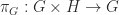
The last example in the previous post said that the collection of all algebraic gadgets of a given kind and structure-preserving maps between them forms a category. The example given was the category of rings. It’s also true that a category itself is an algebraic gadget with structure (the ability to compose morphisms); a structure-preserving map between categories is called a functor. A functor 

- objects of
- morphisms of
such that identities and composition are preserved.
One way of thinking about a functor 
- objects are the eight vertices and
- morphisms are paths along the edges of the cube,


and 
- objects are points of the plane and
- morphisms are paths in the plane,
then a functor 
- each vertex to a point in the plane, and
- each path on the cube to a path in the plane
such that
- composing paths is associative and
- identity paths on the cube map to constant paths in the plane.
These last two requirements imply that the paths in the shadow of the cube are generated by the shadows of each edge.

Illustrated are the images of four functors from the cube 
Exercise: define a functor
Multiplication:composition::monoid:category
The last example in the previous post was the monoid consisting of all functions from a set 

For arbitrary sets, we still know how to compose, but we have some restrictions on what functions are composable: the target of the first has to match the source of the second. Given 


So where multiplication had to start and end at the same place, composition can wander around.
Just as the essence of a monoid is multiplication, the essence of a category is composition.
A category consists of
- a collection of objects and
- for each pair of objects
a set
of morphisms or arrows from
we write
)
such that
- for every object
,
- for every triple of objects
and pair of morphisms
there is a composite morphism
and
- composition is associative
- and obeys the left- and right-unit laws


One simple structure on which something can wander is a directed graph. It has vertices and directed edges between them. We can’t compose two edges and get a new edge, but we can compose two paths and get a new path. Every directed graph gives rise to a category whose objects are the vertices of the graph and whose morphisms are paths in the graph, including “identity paths” that start and end at the same point without going anywhere in between.
Whereas a graph is discrete, a manifold (like a circle or Euclidean space) is continuous. Any manifold gives rise to a category whose objects are the points of the space and whose morphisms are paths between them.
Here are more examples of categories:
1. The empty category:
- no objects
- no morphisms
- one object
- one trivial morphism

3. The category “2”:
- two objects
- the trivial morphisms
and one nontrivial morphism


4. The category Set of all sets:
- objects are sets
- morphisms are functions
- For example,
{1,2} and
{purple, green, yellow} are two objects in Set, and the function
, where
and
is a morphism in

5. Any monoid “is” a one-object category:
- one object
- the set of morphisms from


For example, the real numbers under multiplication form a monoid, so we get a category where
- there’s one object
and
.
- Given
we compose them by multiplying them:

Note:
For example, 


The identity morphism in this case is

Or,
6. Any collection of algebraic gadgets and the structure-preserving maps between them. For example, a ring is an algebraic gadget with two monoids that work together:
- there’s a set
- two different special points, or identities: the multiplicative identity
and the additive identity
- two different associative binary operations
- multiplication:
- addition, which is also commutative:
- multiplication:
- multiplication distributes over addition:


There is a category Ring consisting of all rings and maps between them that preserve the ring structure.
- objects: rings
- morphisms: ring homomorphisms
- A ring homomorphism
is a map between rings that preserves the ring structure: identities, multiplication and addition. That is, it doesn’t matter which way you go around the squares below; the answer will be the same either way:
- For example, the ring of integers
is an object in Ring, as is the ring
(where
denotes integers modulo
The set
where 0 is the ring homomorphism that takes all integers to zero and
is the map that takes each integer to its remainder modulo 2.
- A ring homomorphism


Monoids
A set has no structure. It’s just a collection of things, all of them equally unimportant.

Figure 1. A set.

Figure 2. Another set, the one-element set we’ll call “1.”
A function, or map, “goes between” sets. It has a source set (also called the domain) and a target set (also called the range). To each element of the source set, it assigns an element of the target set. We’ll use the usual shorthand for denoting functions, with the name of the function, a colon, the source set, an arrow, and the target set. Underneath, we’ll write a typical element of the source, an arrow with a small bar at the start, and the element of the target it goes to. For example, consider the function 

Perhaps the simplest structure we can add to a set is to pick an element of it and make that element important. A pointed set
- a set
- a function
, where 1 is the one-element set

The special element of 


A monoid is a pointed set with a little more structure. Way back in kindergarten, they taught us how to count. We counted fingers and marbles and cookies. We used base 1, unary, tally marks:

Sometimes they had us add things that weren’t the same:

Note that when we add this way, the order matters:

While the number of symbols is the same, the result is not!
It takes a long time to teach kids to abstract the concept of a number that’s independent of the order of the symbols in the result. Since that’s one of the earliest things we learn in math, it’s particularly hard to forget, so when anyone says “addition,” we automatically assume it’s commutative. When we get to sticking things like matrices together, there are a couple of natural ways to do it; the commutative way we call “addition,” and the noncommutative one we call “multiplication.”
The only thing a generic monoid knows how to do is stick things together like a kindergartener who hasn’t abstracted the concept of a number yet. Since (in the general case) that’s noncommutative, we call it “multiplication.” When we learned about multiplication in school, we had to memorize our “times table.” The table had numbers across the top and numbers down the sides. Given a row and a column of the table, we could look up the result of multiplying those two numbers.
A “times table” is a function 

So that’s one constraint on the table: multiplying by 

so in our multiplication table, we have

The other constraint on the table is that if you’re multiplying three things, it shouldn’t matter in what order you multiply the pairs. We call this “being associative.” For real numbers, it looks like this:

so in our multiplication table, we have

Now we’re ready for the definition: a monoid consists of a pointed set 
1. The trivial monoid:


2. The free monoid on one element (tally marks under concatenation)
(blank)


3. The whole numbers under addition:

4. The free monoid on two elements (binary strings under concatenation):
where
is the string
followed by the string


5. The reals under multiplication:
- Note: the multiplicative group of real numbers excludes 0, because a group has to have inverses. A monoid does not have to have inverses, so we can include it here.


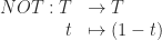
6. Functions from a set
all functions of the form
the identity function
where
is composition of functions:


So, for example, given the set 
00) The constant function mapping everything to zero:01) The identity function:
10) The function that toggles the input:
11) The constant function mapping everything to one:
the identity function


The identity function is the unit for composition:


Exercise: verify that composition is associative.
The partition function and Wick rotation
I was trying to understand Wick rotation by applying it in the case of a finite-dimensional Hilbert space, and came up with something strange. The way I’ve worked it out, it seems to map classical observables to quantum states! I’ve never heard anything like that before.
Say we have an 


where the 
Now define the operators

and 


where the normalizing factor 
- What’s the probability amplitude that when you start in the state
and evolve according to


Except for a factor of 
- What’s the probability amplitude that when you start in the state
Well,
where each
is an arbitrary complex number and
is a normalizing factor. So


If we divide this by the quantity above, we get the expectation value of a classical observable 


This mapping from classical to quantum is not quantization. That maps classical observables to Hermetian operators, not to states—although, one might hit the state with the “Currying” isomorphism between states and linear transformations and get something useful.
I’m trying to work out how to connect this to a sum over paths instead of a sum over states; there’s some interesting stuff there, but I haven’t grokked it yet.

7 comments