SUBJECTIVE EXPLAINER: GUN DEBATE IN THE US
I’m copying this here because I think it’s one of the best explanations of the gun debate I’ve ever read, but Zalewski took down the article. I think I’ve found a couple of the youtube videos he linked to, but the copy of the site I found didn’t copy the links, so I’m just guessing.
2015-10-03 http://lcamtuf.blogspot.com/2015/10/subjective-explainer-gun-debate-in-us.html
In the wake of the tragic events in Roseburg, I decided to briefly return to the topic of looking at the US culture from the perspective of a person born in Europe. In particular, I wanted to circle back to the topic of firearms.
Contrary to popular beliefs, the United States has witnessed a dramatic decline in violence over the past 20 years. In fact, when it comes to most types of violent crime – say, robbery, assault, or rape – the country now compares favorably to the UK and many other OECD nations. But as I explored in my earlier posts, one particular statistic – homicide – is still registering about three times as high as in many other places within the EU.
The homicide epidemic in the United States has a complex nature and overwhelmingly affects ethnic minorities and other disadvantaged social groups; perhaps because of this, the phenomenon sees very little honest, public scrutiny. It is propelled into the limelight only in the wake of spree shootings and other sickening, seemingly random acts of terror; such incidents, although statistically insignificant, take a profound mental toll on the American society. At the same time, the effects of high-profile violence seem strangely short-lived: they trigger a series of impassioned political speeches, invariably focusing on the connection between violence and guns – but the nation soon goes back to business as usual, knowing full well that another massacre will happen soon, perhaps the very same year.
On the face of it, this pattern defies all reason – angering my friends in Europe and upsetting many brilliant and well-educated progressives in the US. They utter frustrated remarks about the all-powerful gun lobby and the spineless politicians, blaming the partisan gridlock for the failure to pass even the most reasonable and toothless gun control laws. I used to be in the same camp; today, I think the reality is more complex than that.
To get to the bottom of this mystery, it helps to look at the spirit of radical individualism and classical liberalism that remains the national ethos of the United States – and in fact, is enjoying a degree of resurgence unseen for many decades prior. In Europe, it has long been settled that many individual liberties – be it the freedom of speech or the natural right to self-defense – can be constrained to advance even some fairly far-fetched communal goals. On the old continent, such sacrifices sometimes paid off, and sometimes led to atrocities; but the basic premise of European collectivism is not up for serious debate. In America, the same notion certainly cannot be taken for granted today.
When it comes to firearm ownership in particular, the country is facing a fundamental choice between two possible realities:
- A largely disarmed society that depends on the state to protect it from almost all harm, and where citizens are generally not permitted to own guns without presenting a compelling cause. In this model, adopted by many European countries, firearms tend to be less available to common criminals – simply by the virtue of limited supply and comparatively high prices in black market trade. At the same time, it can be argued that any nation subscribing to this doctrine becomes more vulnerable to foreign invasion or domestic terror, should its government ever fail to provide adequate protection to all citizens. Disarmament can also limit civilian recourse against illegitimate, totalitarian governments – a seemingly outlandish concern, but also a very fresh memory for many European countries subjugated not long ago under the auspices of the Soviet Bloc.
- A well-armed society where firearms are available to almost all competent adults, and where the natural right to self-defense is subject to few constraints. This is the model currently employed in the United States, where it arises from the straightfoward, originalist interpretation of the Second Amendment – as recognized by roughly 75% of all Americans and affirmed by the Supreme Court. When following such a doctrine, a country will likely witness greater resiliency in the face of calamities or totalitarian regimes. At the same time, its citizens might have to accept some inherent, non-trivial increase in violent crime due to the prospect of firearms more easily falling into the wrong hands.
It seems doubtful that a viable middle-ground approach can exist in the United States. With more than 300 million civilian firearms in circulation, most of them in unknown hands, the premise of reducing crime through gun control would inevitably and critically depend on some form of confiscation; without such drastic steps, the supply of firearms to the criminal underground or to unfit individuals would not be disrupted in any meaningful way. Because of this, intellectual integrity requires us to look at many of the legislative proposals not only through the prism of their immediate utility, but also to give consideration to the societal model they are likely to advance.
And herein lies the problem: many of the current “common-sense” gun control proposals have very little merit when considered in isolation. There is scant evidence that reinstating the ban on military-looking semi-automatic rifles (“assault weapons”), or rolling out the prohibition on private sales at gun shows, would deliver measurable results. There is also no compelling reason to believe that ammo taxes, firearm owner liability insurance, mandatory gun store cameras, firearm-free school zones, bans on open carry, or federal gun registration can have any impact on violent crime. And so, the debate often plays out like this:
[???]
At the same time, by the virtue of making weapons more difficult, expensive, and burdensome to own, many of the legislative proposals floated by progressives would probably gradually erode the US gun culture; intentionally or not, their long-term outcome would be a society less passionate about firearms and more willing to follow in the footsteps of Australia or the UK. Only as we cross that line and confiscate hundreds of millions of guns, it’s fathomable – yet still far from certain – that we would see a sharp drop in homicides.
This method of inquiry helps explain the visceral response from gun rights advocates: given the legislation’s dubious benefits and its predicted long-term consequences, many pro-gun folks are genuinely worried that making concessions would eventually mean giving up one of their cherished civil liberties – and on some level, they are right.
Some feel that this argument is a fallacy, a tell tale invented by a sinister corporate “gun lobby” to derail the political debate for personal gain. But the evidence of such a conspiracy is hard to find; in fact, it seems that the progressives themselves often fan the flames. In the wake of Roseburg, both Barack Obama and Hillary Clinton came out praising the confiscation-based gun control regimes employed in Australia and the UK – and said that they would like the US to follow suit. Depending on where you stand on the issue, it was either an accidental display of political naivete, or the final reveal of their sinister plan. For the latter camp, the ultimate proof of a progressive agenda came a bit later: in response to the terrorist attack in San Bernardino, several eminent Democratic-leaning newspapers published scathing editorials demanding civilian disarmament while downplaying the attackers’ connection to Islamic State.
Another factor that poisons the debate is that despite being highly educated and eloquent, the progressive proponents of gun control measures are often hopelessly unfamiliar with the very devices they are trying to outlaw:
I’m reminded of the widespread contempt faced by Senator Ted Stevens following his attempt to compare the Internet to a “series of tubes” as he was arguing against net neutrality. His analogy wasn’t very wrong – it just struck a nerve as simplistic and out-of-date. My progressive friends did not react the same way when Representative Carolyn McCarthy – one of the key proponents of the ban on assault weapons – showed no understanding of the supposedly lethal firearm features she was trying to eradicate. Such bloopers are not rare, too; not long ago, Mr. Bloomberg, one of the leading progressive voices on gun control in America, argued against semi-automatic rifles without understanding how they differ from the already-illegal machine guns:
Yet another example comes Representative Diana DeGette, the lead sponsor of a “common-sense” bill that sought to prohibit the manufacture of magazines with capacity over 15 rounds. She defended the merits of her legislation while clearly not understanding how a magazine differs from ammunition – or that the former can be reused:
“I will tell you these are ammunition, they’re bullets, so the people who have those know they’re going to shoot them, so if you ban them in the future, the number of these high capacity magazines is going to decrease dramatically over time because the bullets will have been shot and there won’t be any more available.”
Treating gun ownership with almost comical condescension has become vogue among a good number of progressive liberals. On a campaign stop in San Francisco, Mr. Obama sketched a caricature of bitter, rural voters who “cling to guns or religion or antipathy to people who aren’t like them”. Not much later, one Pulitzer Prize-winning columnist for The Washington Post spoke of the Second Amendment as “the refuge of bumpkins and yeehaws who like to think they are protecting their homes against imagined swarthy marauders desperate to steal their flea-bitten sofas from their rotting front porches”. Many of the newspaper’s readers probably had a good laugh – and then wondered why it has gotten so difficult to seek sensible compromise.
There are countless dubious and polarizing claims made by the supporters of gun rights, too; examples include a recent NRA-backed tirade by Dana Loesch denouncing the “godless left”, or the constant onslaught of conspiracy theories spewed by Alex Jones and Glenn Beck. But when introducing new legislation, the burden of making educated and thoughtful arguments should rest on its proponents, not other citizens. When folks such as Bloomberg prescribe sweeping changes to the American society while demonstrating striking ignorance about the topics they want to regulate, they come across as elitist and flippant – and deservedly so.
Given how controversial the topic is, I think it’s wise to start an open, national conversation about the European model of gun control and the risks and benefits of living in an unarmed society. But it’s also likely that such a debate wouldn’t last very long. Progressive politicians like to say that the dialogue is impossible because of the undue influence of the National Rifle Association – but as I discussed in my earlier blog posts, the organization’s financial resources and power are often overstated: it does not even make it onto the list of top 100 lobbyists in Washington, and its support comes mostly from member dues, not from shadowy business interests or wealthy oligarchs. In reality, disarmament just happens to be a very unpopular policy in America today: the support for gun ownership is very strong and has been growing over the past 20 years – even though hunting is on the decline.
Perhaps it would serve the progressive movement better to embrace the gun culture – and then think of ways to curb its unwanted costs. Addressing inner-city violence, especially among the disadvantaged youth, would quickly bring the US homicide rate much closer to the rest of the highly developed world. But admitting the staggering scale of this social problem can be an uncomfortable and politically charged position to hold. For Democrats, it would be tantamount to singling out minorities. For Republicans, it would be just another expansion of the nanny state.
PS. If you are interested in a more systematic evaluation of the scale, the impact, and the politics of gun ownership in the United States, you may enjoy an earlier entry on this blog. Or, if you prefer to read my entire series comparing the life in Europe and in the US, try this link.
Dependent types and function bivariance
TypeScript is unsound in part because of a desire to avoid forcing programmers to write a cast with no runtime effect just to satisfy the type checker. This code comes from their documentation on the unsoundness:
enum EventType {
  Mouse,
  Keyboard,
}

interface Event {
  timestamp: number;
}
interface MyMouseEvent extends Event {
  x: number;
  y: number;
}
interface MyKeyEvent extends Event {
  keyCode: number;
}

function listenEvent(eventType: EventType, handler: (n: Event) => void) {
  /* ... */
}

// Unsound, but useful and common
listenEvent(EventType.Mouse, (e: MyMouseEvent) => console.log(e.x + "," + e.y));

// Undesirable alternatives in presence of soundness
listenEvent(EventType.Mouse, (e: Event) =>
  console.log((e as MyMouseEvent).x + "," + (e as MyMouseEvent).y)
);
listenEvent(EventType.Mouse, ((e: MyMouseEvent) =>
  console.log(e.x + "," + e.y)) as (e: Event) => void);

// Still disallowed (clear error). Type safety enforced for wholly incompatible types
listenEvent(EventType.Mouse, (e: number) => console.log(e));
However, TypeScript now supports a restricted notion of dependent type, so the motivating example is no longer a problem:
// Assuming EventType, Event, MyMouseEvent, and MyKeyEvent as above

type GenericEvent<E extends EventType> = E extends EventType.Mouse ? MyMouseEvent : MyKeyEvent

function listenEvent<E extends EventType>(eventType: E, handler: (n: GenericEvent<E>) => void): void;
function listenEvent(eventType: EventType, handler: (n: GenericEvent<typeof eventType>) => void): void {
  /* ... */
}

// Valid
listenEvent(EventType.Mouse, (e: MyMouseEvent) => console.log(e.x + "," + e.y));
// Valid
listenEvent(EventType.Keyboard, (e: MyKeyEvent) => console.log(e.keyCode));
// Invalid
listenEvent(EventType.Mouse, (e: MyKeyEvent) => console.log(e.keyCode));
// Invalid
listenEvent(EventType.Mouse, (e: Event) => console.log(e.x + "," + e.y));
Dependent types don’t solve all the usability issues preventing soundness, but they remove a major one, and libraries should be updated to take advantage of dependent types.
A Modest Proposal for Operator Overloading in JavaScript
It is a melancholy object-oriented language to those who walk through this great town or travel in the country, when they see the JavaScript programs crowded with method calls begging for more succinct syntax. I think it is agreed by all parties, that whoever could find out a fair, cheap and easy method of making these operators sound and useful members of the language, would deserve so well of the publick, as to have his statue set up for a preserver of the nation. I do therefore humbly offer to publick consideration a pure JavaScript library I have written for overloading operators, which permits computations like these:
Complex numbers:
>> Complex()({r: 2, i: 0} / {r: 1, i: 1} + {r: -3, i: 2})
<- {r: -2, i: 1}
Automatic differentiation: Let

>> var f = x => Dual()(x * x * x - {x:5, dx:0} * x);
Now map it over some values:
>> [-2, -1, 0, 1, 2].map(a=>({x:a, dx:1})).map(f).map(a=>a.dx)
<- [ 7, -2, -5, -2, 7 ]
i.e.
Polynomials:
>> Poly()([1, -2, 3, -4]*[5, -6]).map((coeff, pow)=>'' + coeff + 'x^' + pow).join(' + ')
<- "5x^0 + -16x^1 + 27x^2 + -38x^3 + 24x^4"
Big rational numbers:
>> // 112341324242 / 22341234124 + 334123124 / 5242342
>> with(Rat){Rat()(n112341324242d22341234124 + n334123124d5242342).join(' / ')}
<- "2013413645483934535 / 29280097495019602"
Monadic bind:
>> Bind()([5] * (x => [1,2,3].map(y => x * y)) * (x => [4,5,6].map(y => x * y)))
<- [20, 25, 30, 40, 50, 60, 60, 75, 90]
The implementation is only mildly worse than eating babies.
How does it work?
There are four cunning devices at play here. The first is one that various others have discovered: the arithmetic operators do coersion on their operands, and if the operand is an object (as opposed to a primitive), then its valueOf method gets invoked. The question then becomes, “What value should valueOf return?” The result of coersion has to be a number or a string, and multiplication only works with numbers, so we have to return a number.
People have tried packing data about the operand into JavaScript’s IEEE 754 floats, but they only hold 64 bits. Wherefore, if you have a Point(x, y) class, then you can represent it as the number x * 10**12 + y or some such, but the points have much more limited precision and you can only add and subtract them. This is almost useless for polynomials.
The second device is to have the valueOf method store this in a table (line 87) and use the result of the expression to figure out what to do with the values in the table. Others have also discovered this before. By means of this device, we get to store all the information about the objects we are manipulating, but it is still unclear what number to return. This good fellow uses the number 3 to be able to do a single subtraction, a single division, multiple additions, or multiple multiplications.
The third device allows us to use arbitrary expressions. It depends on an observation from abstract algebra: numbers chosen uniformly at random from the unit interval are transcendental with probability 1. That implies there are no two fundamentally different arithmetic expressions using each random number once and the operators for addition, subtraction, multiplication, and division that have the same value. With IEEE 754 floats, one can uniquely distinguish nearly 2**64 different expressions by their result. I enumerate all possible arithmetic expressions in numVars variables (lines 13–30 enumerate the structure of the abstract syntax tree, while lines 32–42 turn it into JavaScript), evaluate the expression with the variables set to the random numbers, and store the expression in a table under the result (54–77).
There is a complication in that JavaScript has operator precedence: in the expression 3-4*5, the multiplication is done first and then the subtraction. Wherefore, in evaluating the expression, I have to keep track of the order in which objects get coerced (60–61). When I get the coerced result of an expression, I look up the original expression in the table (90–91), permute the objects based on the order they get coerced (96), and then execute the expression with the appropriate methods corresponding to +-*/ (97).
The last device gets used in Str and Rat above. In a with block of the form with(obj){ body }, if a variable name mentioned in body is a property name of obj, then the property is returned. I use a Proxy for obj (138, 162) with handlers that claim every possible property of a certain form (the has method on lines 142 and 168). Str claims to have all properties that match the regex /^[a-z0-9A-Z_]+$/ other than Str, while Rat claims to have all properties that match the regex /^n([0-9]+)d([0-9]+)$/ (a numerator followed by a denominator). When asked what value those variables have, the Proxy responds with the appropriate data structure: Str says the value of prop is [prop] (145), while Rat says the value of n<numerator>d<denominator> is the pair [<numerator>, <denominator>], where I use BigInt to make sure there’s no loss in precision and reduce so the fraction is always in lowest form (172).
I profess in the sincerity of my heart, that I have not the least personal interest in endeavouring to promote this necessary work, having no other motive than the publick good of my community, by advancing our trade and giving some pleasure to the front-end developer.
((global) => {
  // Increase for more complicated fancier expressions
  var numVars = 5;


  var vars = Array.from(Array(numVars)).map((_,i)=>i);
  var randoms = vars.map(() => Math.random());
  var table = {};

  // n is number of internal nodes
  // f is a function to process each result
  var trees = (n, f) => {
    // h is the "height", thinking of 1 as a step up and 0 as a step down
    // s is the current state
    var enumerate = (n, h, s, f) => {
      if (n === 0 && h === 0) {
        f(s + '0');
      } else {
        if (h > 0) {
          enumerate(n, h - 1, s + '0', f)
        }
        if (n > 0) {
          enumerate(n - 1, h + 1, s + '1', f)
        }
      }
    };

    enumerate(n, 0, '', f);
  };

  var toFunction = (s, pos, opCount, varCount) => {
    if (s[pos] == '0') {
      return [`x[${varCount}]`, pos + 1, opCount, varCount + 1];
    }
    var left, right, op;
    pos++;
    op = `ops[${opCount}]`;
    [left, pos, opCount, varCount] = toFunction(s, pos, opCount + 1, varCount);
    [right, pos, opCount, varCount] = toFunction(s, pos, opCount, varCount);
    return [`${op}(${left},${right})`, pos, opCount, varCount];
  };

  var add = (x,y) => x+y; add.toString = ()=>'+';
  var sub = (x,y) => x-y; sub.toString = ()=>'-';
  var mul = (x,y) => x*y; mul.toString = ()=>'*';
  var div = (x,y) => x/y; div.toString = ()=>'/';

  var round = (x) => {
    var million = Math.pow(2,20);
    return Math.floor(x * million) / million;
  };

  var populate = (expr, ops, opCount) => {
    if (ops.length == opCount) {
      var result;
      var order=[];
      var x = vars.map(y => ({
        valueOf:()=>{
          order.push(y);
          return randoms[order.length - 1];
        }
      }));
      with ({ops, x}) { result = round(eval(expr)); }
      table[result] = {ops: ops.map(x => '' + x), expr, order};
    } else {
      populate(expr, ops.concat(add), opCount);
      populate(expr, ops.concat(sub), opCount);
      populate(expr, ops.concat(mul), opCount);
      populate(expr, ops.concat(div), opCount);
    }
  };

  var allExprs = (s) => {
    var [expr, , opCount, ] = toFunction(s, 0, 0, 0);
    populate(expr, [], opCount);
  };

  vars.forEach(x=>trees(x, allExprs));

  var makeContext = (constrs, opTable) => () => {
    // Set up values array
    var V = [];
    // Install temporary valueOf
    var valueOf = constrs.map(c => c.prototype.valueOf);
    constrs.forEach(c => c.prototype.valueOf = function () {
      return randoms[V.push(this) - 1];
    });
    // Return function expecting key
    return (key) => {
      var {ops, expr, order} = table[round(+key)];
      constrs.forEach((c, i) => c.prototype.valueOf = valueOf[i]);
      var result;
      var index = 0;
      var W = [];
      V.forEach((v, i) => W[order[i]] = V[i]);
      with ({ops: ops.map(x => opTable[x]), x: W}) { result = eval(expr); }
      V = [];
      return result;
    };
  };
  global.makeContext = makeContext;
})(this);

var Complex = makeContext([Object], {
  '+': (x, y) => ({r: x.r + y.r, i: x.i + y.i}),
  '-': (x, y) => ({r: x.r - y.r, i: x.i - y.i}),
  '*': (x, y) => ({r: x.r * y.r - x.i * y.i, i: x.r * y.i + x.i * y.r}),
  '/': (x, y) => {
    const norm = y.r**2 + y.i**2;
    return {r: (x.r * y.r + x.i * y.i) / norm, i: (x.i * y.r - x.r * y.i) / norm};
  }
});

var Dual = makeContext([Object], {
  '+': (a, b) => ({x: a.x + b.x, dx: a.dx + b.dx}),
  '-': (a, b) => ({x: a.x - b.x, dx: a.dx - b.dx}),
  '*': (a, b) => ({x: a.x * b.x, dx: a.x * b.dx + a.dx * b.x}),
  '/': (a, b) => ({x: a.x / b.x, dx: (a.dx * b.x - a.x * b.dx) / (b.x ** 2)})
});

var Poly = makeContext([Array], {
  '+': (a, b) => (a.length >= b.length ? a.map((x,i) => x + (b[i]?b[i]:0)) : b.map((x,i) => x + (a[i]?a[i]:0))),
  '-': (a, b) => (a.length >= b.length ? a.map((x,i) => x - (b[i]?b[i]:0)) : b.map((x,i) => x - (a[i]?a[i]:0))),
  '*': (a, b) => {
    var result = [];
    for (var i = 0; i < a.length; ++i) {
      for (var j = 0; j < b.length; ++j) {
        result[i+j] = result[i+j] ? result[i+j] : 0;
        result[i+j] += a[i] * b[j];
      }
    }
    return result;
  },
  '/': (a, b) => { throw new Error('Not implemented'); }
});

var Str = new Proxy(makeContext([Array], {
  '+':(a,b) => [a[0]+b[0]],
  '*':(a,b) => [Array.from(Array(b[0])).map(x=>a[0]).join('')]
}), {
  has (target, key) { return key.match(/^[a-z0-9A-Z_]+$/) && key !== 'Str'; },
  get(target, prop, receiver) {
    if (typeof prop == 'string') {
      return [prop];
    } else {
      return target[prop];
    }
  }
});

function reduce(numerator,denominator) {
  var gcd = function gcd(a, b){
    return b ? gcd(b, a % b) : a;
  };
  gcd = gcd(numerator, denominator);
  return [numerator/gcd, denominator/gcd];
}

var numDenom = /^n([0-9]+)d([0-9]+)$/;

var Rat = new Proxy(makeContext([Array], {
  '+':(a,b) => reduce(a[0]*b[1] + a[1]*b[0], a[1]*b[1]),
  '-':(a,b) => reduce(a[0]*b[1] - a[1]*b[0], a[1]*b[1]),
  '*':(a,b) => reduce(a[0]*b[0], a[1]*b[1]),
  '/':(a,b) => reduce(a[0]*b[1], a[1]*b[0])
}), {
  has (target, key) { return !!key.match(numDenom); },
  get(target, prop, receiver) {
    if (typeof prop == 'string') {
      var m = prop.match(numDenom);
      return reduce(BigInt(m[1]), BigInt(m[2]));
    } else {
      return target[prop];
    }
  }
});

var Sets = makeContext([Set], {
  // disjoint union
  '+': (a, b) => new Set([...[...a].map(v=>[0,v]), ...[...b].map(v=>[1,v])]),
  // product
  '*': (a, b) => new Set([...a].flatMap(v => b.map(w => [v, w]))),
});

var Inj = makeContext([Set], {
  // union
  '+': (a, b) => new Set([...a, ...b]),
  // difference
  '-': (a, b) => new Set([...a].filter(v => !b.has(v))),
  // intersection
  '*': (a, b) => new Set([...a].filter(v => b.has(v))),
});

var Bind = makeContext([Object, Array, Function], {
  '*': (a, b) => a.flatMap(b)
});

Mrs. Wingate
When I was a senior in high school, I had calculus right after lunch. The room was also on the west side of the building, so the combination of dense math, a full belly, and the warm sun often conspired to make me fall asleep. One day woke up and didn’t understand a term my teacher, Mrs. Wingate, was using. It was a word I knew—”normal”—but in a way I’d never heard it. I raised my hand to ask what it meant, and she replied, “Mike, go back to sleep.” The reason she was so forgiving was apparently because I was the only one in the class who came in after school to ask more questions. Some she knew how to answer, like how to calculate the surface volume of a hypersphere. Others she didn’t, like, whether you can raise an imaginary number to an imaginary power—but she dug through her files and found me an article on polar coordinates and Euler’s formula. She had a small library of mathematical books. I borrowed a book of mathematical fiction; it was volume 4 in some series, bound in navy blue with an infinity symbol on the spine. It had one story about a device to twist things into a fourth dimension for (among other things) robbing bank vaults; there was another about a topologist who, dissatisfied with the Möbius strip’s single side, discovered a complicated topological surface with no sides—but whenever he tried to make one out of paper, it would disappear. She also had a book about flexagons. When she retired, she gave my family the book on flexagons, because every one of my five younger siblings also borrowed the book and no other students ever had. She taught us so well that taking the AP calculus exam was a downright enjoyable experience. I can’t thank her enough for leading me to one of the principal joys of my life.
Anomalous magnetic moment still anomalous
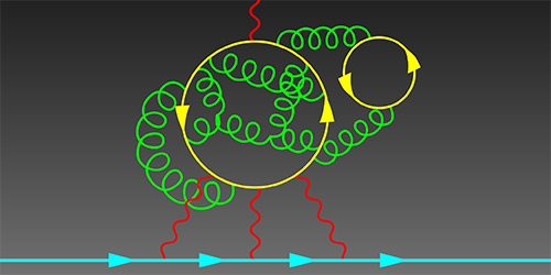
Supercomputer simulations show effect of hadron light-by-light scattering is far too small to account for the 3.7σ deviation from Standard Model predictions. There’s still hope for new physics at accessible energies!
How we recovered over $300K of Bitcoin
Story time! Around twenty years ago, I was working as a reverse-engineer and cryptanalyst for AccessData while getting my Physics degree at BYU. It was the late 90s and early 2000s. The US government had been gradually easing off export restrictions on software containing cryptography, but most software still contained pretty worthless password protection. We’d buy desktop office software, I’d reverse-engineer it to figure out what algorithm it was using for access control, and then break the crypto. It was a never-ending stream of interesting-but-not-impossible math puzzles. I wrote about forty password crackers during my time there. We would sell them to home users, system administrators, and local and federal law enforcement agencies. I got to go down to the Federal Law Enforcement Training Center in Glynco a few times to teach the Secret Service, FBI, and ATF about cryptography and the use of our products.
Two projects really stand out in my memory. The first was Microsoft Word 97. Before Word 97, the files were encrypted by xoring the bytes with a repeating 16-byte string derived from the password. The most common bytes in a Word file were usually either 0x00, 0xFF, or 0x20 (space), so we’d just look at the most common character in each column and try the 316 variations on those. Recovering the key was usually instantaneous, but to help people feel like they’d gotten their money’s worth, we’d put on a little animated show like a Hollywood hacking scene with lots of random characters that gradually revealed the right password.
Microsoft 97 changed that. It might have been possible to find out the encryption format through MSDN, but we were small and couldn’t afford a subscription. It also wasn’t clear that we’d be allowed to write the cracker if we did get the info from them. To figure out how it worked, I used SoftICE to stop the software immediately after typing in the password, then walked slowly up the stack until I could find the algorithm. This was before IDA Pro, so I printed out a few dozen pages of assembly code, taped it to the wall, and drew all over it with a red crayon. I was very pleased when I finally worked it all out. At the time, Microsoft was only allowed to export 40 bit cryptography, so they did as much as they were legally permitted: they’d repeatedly MD5 hash the password with “salt” (randomly chosen bytes stored in the file) to get the 40 bit key, then add salt to that and repeatedly hash it again. It took roughly half a second to test a password on the computers of the time. We had to resort to a dictionary attack, because breaking it outright was pretty much impossible. We did eventually write a cracker for larger companies and agencies that brute-forced the 40-bit keyspace using those fancy MMX instructions on the Pentium. I knew of one place that ran the software for nine months before finally getting in.
The other really fun one one was zip archives. The developer of PKZIP, Phil Katz, made the decision—unusual at the time—to document his file format and include it with his software, making it a favorite of developers. Roger Schlafly designed the stream cipher used for encrypting the archives. The zip standard quickly became by far the most popular compression format on Windows, and many other formats like Java’s .jar format and OpenOffice’s document formats are really zip files with a particular directory structure inside. InfoZIP is an open-source version of the software; its implementation was used as the basis for nearly all other branded zip software, like WinZip. At the time I was trying to crack it, WinZip had 95% of the market.
Eli Biham and Paul Kocher had published a known-plaintext attack on the cipher, but the known plaintext was compressed plaintext. To get the Huffman codes at the start of a deflated file, you basically need the whole file. The attack was practically useless to law enforcement agencies.
The zip cipher has 96 bits of internal state split into three 32-bit chunks called key0, key1, and key2. key0 and key2 are the internal state of two copies of CRC32, a linear feedback shift register. Basically, to update the state with a new byte of data, you shift all the bytes down by one byte (dropping the low byte) then xor in a constant from a lookup table indexed by the byte of data xored with the low byte. key1 is the internal state of a truncated linear congruential generator (TLCG). To update its internal state, you add the data byte, multiply by a constant I’ll call c, and add 1. The cipher works like this: you feed in a data byte to the first CRC32, then take the low byte of that and feed it into the TLCG, then take the high byte of that and feed it into the second CRC32, then take the state and (roughly) square it, then output the second byte of the result as the stream byte. To initialize the 96-bit state, you start from a known state and encrypt the password, then encrypt ten bytes of salt.
PKZIP got its salt bytes by allocating memory without initializing it, so it would contain bits of stuff from other programs you’d been running or images or documents, whatever. That worked fine on Windows, but on many Unix systems, memory gets initialized automatically when it’s allocated. InfoZIP chose the salt bytes by using C’s rand function. It would initialize the state of the random number generator by xoring the timestamp with the process ID, then generate ten bytes per file. Had they left it that way, knowing the timestamp and process ID would be enough information to recover the header bytes, which in turn would let you mount Biham and Kocher’s attack. It seems the InfoZIP authors knew about that attack, because they went one step further and encrypted the headers once using the password. That way an attacker had only doubly-encrypted plaintext, and their attack wouldn’t work.
I noticed that because the password was the same in both passes, the first stream byte was the same each pass. Just like toggling a light switch twice leaves it where it started, xoring a byte twice with the same stream byte leaves it unaffected. This let me mount a very powerful ciphertext only attack: given five encrypted files in an archive, I could derive the internal state of C’s rand function without having to look at the timestamp or knowing the process ID. That let me generate the original, unencrypted headers. Because only a few bits of each part of the cipher affected the next part, I could also guess only a few bits of the state and check whether decrypting the next bytes twice gave me the answer I was expecting. I had to guess fewer and fewer bits of key material as I went on. Each extra file also let me exclude more potential key material; at the time, it took a few hours on a single desktop machine. I published a paper on it and got to present it in Japan at Fast Software Encryption 2001.
I left AccessData in 2002. I worked for a neural networking startup for a year, spent three years on a Master’s degree in Computer Science at the University of Auckland with Cris Calude, started a PhD with the mathematical physicist John Baez at UC Riverside, worked on Google’s applied security team for six years and finished the PhD, and after a few more years ended up as CTO of a startup.
About six months ago, I received, out of the blue, a message on LinkedIn from a Russian guy. He had read that paper I’d written 19 years ago and wanted to know if the attack could work on a file with only two files. A quick analysis said not without an enormous amount of processing power and a lot of money. Because I only had two files to work with, a lot more false positives would advance at each stage. There would end up being 273 possible keys to test, nearly 10 sextillion. I estimated it would take a large GPU farm a year to break, with a cost on the order of $100K. He astounded me by saying he could spend that much to recover the key.
Back in January of 2016, he had bought around $10K or $15K of Bitcoin and put the keys in an encrypted zip file. Now they were worth upwards of $300K and he couldn’t remember the password. Luckily, he still had the original laptop and knew exactly when the encryption took place. Because InfoZip seeds its entropy using the timestamp, that promised to reduce the work enormously—”only” 10 quintillion—and made it quite feasible, a matter of a couple of months on a medium GPU farm. We made a contract and I got to work.
I spent a while reconstructing the attack from the overview in the paper. To my chagrin, there were certain tricky details I had skimmed over in my paper, but I worked them out again. Then I discovered I’d made a terrible mistake while estimating the work!
In my original attack, I would guess the high bytes of key1·c, key1·c², key1·c³, and key1·c⁴. By the time I guessed that fourth byte, I knew the complete state of the rest of the cipher; I just had to convert those four bytes into the original key1 and I was done. I would run through the 32-bit state space for key1 and check each one to see if it gave the proper high bytes. Here, though, I had quintillions of keys to check; if I had to do 232 tests on each one, it would take a few hundred thousand years.
I vaguely remembered that there had been some work done on cryptanalyzing TLCGs using lattice reduction, so I dug out the original paper. It was perfect! I just needed to define a lattice with basis vectors given by 232 and the powers of the constant from the TLCG, then do lattice reduction. Given the reduced basis, I could recover the original state from the high bytes just by doing a matrix multiplication.
At least, that was the idea. I would need five bytes to constrain it to a single outcome, and at that point in the attack, I only had four. The process described in the paper rarely gave the right answer. However, I knew the answer had to be close to the right one, so I ran through all the possible key1 values and checked the difference from the answer it gave me and the true one. The difference was always one of 36 vectors! With this optimization, I could run through just 36 possibilities instead of four billion. We were still in business.
The next thing we ran into was the problem of transferring data between the machines with the GPUs on them. My business partner, Nash Foster, was working on the GPU implementation, advising me on how fast different operations are and writing a lot of the support structure for the application into which I put my crypto cracking code. How would we get these petabytes of candidate keys to the GPUs that would test them? They’d be almost idle, twiddling their thumbs waiting for stuff to work on. It occurred to me that each stage of my attack was guessing a lot of bits and then keeping only one candidate out of roughly 65K. If I had some way of using that information to derive bits rather than just guess and check, I’d save a lot of work, and more importantly, a lot of network traffic. The problem with that idea was that the math was too complicated; it involved mixing the math of finite fields with the math of integer rings, and those don’t play nicely together.
I thought about other cryptanalytic attacks I knew, and one that seemed promising was a meet-in-the-middle attack. A meet-in-the-middle attack applies to a block cipher when it uses one part of the key material to do the first half of the encryption and the other part of the key material to do the second half. That sort-of applied to the zip cipher, but the key material far outweighed the number of bits in the middle. Then it occurred to me that I could use the linearity of CRC32 to my advantage: by xoring together two outputs of the last CRC32, the result would be independent of key2! Rather than compute the intermediate state of the cipher and store it in a table, I’d calculate the xor of two intermediate states and store that instead.
I wrote up the differential meet-in-the-middle attack and ran it on my laptop. A stage that had taken hours on my laptop before now finished in mere seconds. The next stage, which I expected to take a week on the GPU farm finished in a few hours on a powerful CPU. I couldn’t quite make it work fast enough on the third stage to be useful in speeding up the overall attack, but it completely obviated the need to move data around: we simply computed the candidates for each GPU on the computer with the cards in it. Nash wrote the GPU code, which ran screamingly fast.
The attack ran for ten days and failed.
I was heartbroken. Had we missed one of the candidate keys? We went back and looked at the maximum process ID on his laptop and discovered it was a few bits larger than we had expected, and therefore there were a couple of other possible initial seeds for rand. I also went back and double-checked all our tests. Was there something we’d missed? Did the CPU-based version behave any differently from the GPU version? Our client was re-running our tests and discovered that the GPU version failed to find the correct key when it was the second in a list of candidates, but it worked when it was the first one. Digging into the code, we found that we had swapped the block index with the thread index in computing the offset into the data structure.
We fixed the bug, re-ran the code, and found the correct key within a day. Our client was very happy and gave us a large bonus for finding the key so quickly and saving him so much money over our initial estimate.
I’m currently looking for work in a staff or senior staff engineering or data scientist role. If you’ve got interesting technical analysis or optimization problems, please reach out to me and let’s talk.
Clinical trial of CRISPR-based cure for sickle cell anemia shows promise

They extracted stem cells, used electrophoresis to open up pores in the cells, CRISPR to turn off the DNA switch that stops the production of fetal red blood cells (which are always made correctly), turned the stem cells into marrow cells, killed the bone marrow in the patient (!), and repopulated the bones with the new marrow.


D-Day exhibit at Bletchley Park
Rose Design did some really lovely work for the design of the 75th anniversary of D-Day exhibit at Bletchley Park. The D itself was made from ticker tape; they used the ITA2 Boudot-Murray teletype standard to type the words “Interception Intelligence Invasion” (interspersed with NULs to make it more aesthetically pleasing):


I had hoped they’d encrypted the words with the Lorenz SZ-40 cipher, used by German High Command, which Colossus was created to break. But ITA2 is certainly much cooler than A=1, B=2, etc.


Sonorous rocks
http://www.geologyin.com/2019/07/ringing-rocks-geological-and-musical.html
A more plausible theory is that the elastic stresses remained in the rock when the boulder fields formed, and the slow weathering rate keeps the stresses from dissipating. A possible source of the stresses would likely be the loading stresses from the time when the rock crystallized. The diabase sill formed at roughly 1.2–1.9 miles (2–3 km) beneath the surface.
This “relict stress” theory implies that the ringing rock boulders act much like a guitar string. When a guitar string is limp it does not resonate, but a plucked string will provide a range of sounds depending on the level of applied tension.
Obligatory:


Using EEG and TMS for low-bandwidth telepathy
EEG on people staring at flashing lights can pick up difference between different frequencies. TMS can create phosphenes. These guys hooked them together and played Tetris.
https://www.sciencealert.com/brain-to-brain-mind-connection-lets-three-people-share-thoughts

At least three different times, crocodiles evolved to become herbivores

Comments Off on At least three different times, crocodiles evolved to become herbivores

Borneo earless monitors look the most like fantasy dragons

Followed closely by the armadillo girdled lizard:

Text generators
In the last year, enormous progress has been made in generating coherent text.
https://minimaxir.com/apps/gpt2-small/ A model less than a tenth the size of the 1.5B GPT2 model that the researchers are refusing to release. Dreamlike, choppy, somewhat incoherent, but an order of magnitude better than what we had last year.
https://grover.allenai.org/ – type in a headline, then hit “generate” on the body box. Grover was designed to distinguish fake news from real news, so it knows how to avoid the problems that plague gpt2-small. This stuff is just barely distinguishable from human authorship.
Analysis says there are four different kinds of sepsis that need to be treated differently
Using a combination of statistical, machine learning, and simulation tools, the researchers combed through data relating to 20,000 past hospital patients who had developed sepsis within six hours of admission.
In particular, they looked for clusters of symptoms and patterns of organ dysfunction, then correlated them against biomarkers and mortality.
The findings revealed not one discernible type of sepsis, but four, which the researchers label alpha, beta, gamma and delta.
Alpha sepsis was the most common, affecting 33% of patients, and carried the lowest fatality rate, about 2%. At the other end of the scale, delta sepsis occurred in only 13% of patients, but had an in-hospital death rate of 32%.
To further test their discovery, Seymour and colleagues ran the same analysis on records for a further 43,000 patients, all of whom had been treated for sepsis between 2012 and 2014. The finding held.
https://cosmosmagazine.com/biology/sepsis-treatments-wrong-by-definition-study-finds
Pluto may have subsurface ocean insulated by clathrates
Popular account: “And if Pluto has such materials, it stands to reason that other outer solar system bodies also have them, including not only the moons of Jupiter and Saturn, but possibly other large Kuiper Belt objects, even farther out from the sun than Pluto.”
https://cosmosmagazine.com/space/pluto-has-an-insulated-underground-ocean
Nature article:
https://www.nature.com/articles/nature20148
Latest claim: Voynich manuscript was written in proto-Romance
https://www.tandfonline.com/doi/full/10.1080/02639904.2019.1599566
Edit: Aaand now it’s been withdrawn.

Each one had six wings; with twain he covered his face, and with twain he covered his feet, and with twain he did fly.
All insects have two pairs of wings, sprouting from the second and third segment of the thorax. Even insects that appear to have only one pair, like flies and beetles, really have two: in flies, the second pair of wings diminished to new structures called halteres, while in beetles, the first pair became the elytra. In cockroaches and bugs, the first pair only got halfway to elytra and are called hemelytra.
But! A 2011 paper in Nature gives morphological and genetic evidence that the helmet of treehoppers is derived from a third pair of wing buds on the first segment. Hox genes have suppressed wing expression on every segment but 2 and 3 for 300 million years. Hox genes control repetition of certain body parts. They are very strongly preserved, since they govern the gross body plan of a creature—in humans, for instance, they control how many vertebrae we have. The authors suspected that the treehopper hox gene no longer suppressed production on the first gene and inserted it into drosophila flies to see if wing primordia formed, but they didn’t. So somehow, despite the hox genes being preserved, treehoppers found a way around the inhibition of wing production and were able to evolve their fantastic helmets.

TIL: Till is not a shortening of until
‘Til is a corruption of till under the assumption that it is a shortening of until, but till is, in fact, an older word than until. Both till and until mean the same thing.
Journey to the black hole at the center of the galaxy
Here’s some context for the recent black hole image.
Shock diamonds and aerospikes
I was curious what caused the oscillations in rocket exhaust. I learned they’re called “shock diamonds”, among other names, and are due to the lateral pressure of the exhaust being mismatched with the atmospheric pressure. At low altitudes / high pressure, the exhaust is immediately pinched and then bounces off itself as the pressure increases, then becomes repinched as it expands again. At high altitudes / low pressure, the exhaust expands first, then gets pinched at the lower pressure. The bell-style rocket only has its maximum efficiency at one specific altitude; this is one reason for multistage rockets.

There’s a rocket design called an aerospike that effectively uses air for half the bell and then controls the flow to match the air pressure. It’s more efficient, but has had bad luck as far as deployment goes. Since fuel is about the cheapest part of a rocket, new space companies have opted for using known, proven designs instead. This is a good video about the history and development of the aerospike.
While looking for the explanation, I came across this wonderful paper that examines what happens when two laminar flows collide. Depending on the viscosity, surface tension, and velocity of the streams, you get several different “phases” of interaction.

Lightfield 3d photos from an inkjet!
Lumii uses multilayer Moire patterns to simulate lightfields. You print out the layers on a regular transparency from an inkjet printer!

Fantastic fossil find from dinosaur killer asteroid
Seismic waves from the Chicxulub impact set up enormous standing waves in a large inland sea in North Dakota. The waves hit the mouth of an incoming river, which focused the waves into a 30 foot wall of water that knocked down trees and put fish next to triceratops and hadrosaurs in the fossil bed. The fish’s gills were also clogged with tektites, ejecta from the impact made of hot glass spherules that set the world’s forests on fire.
https://news.berkeley.edu/2019/03/29/66-million-year-old-deathbed-linked-to-dinosaur-killing-meteor/?T=AU

JavaScript can’t be fixed
In 2015, Andreas Rossberg of the V8 team proposed making JavaScript a little saner by making classes, objects, and functions unalterable after their construction so that a sound type system becomes possible.
A year later, his team reported on their progress and said that there’s basically no way to do that without breaking compatibility with everything that came before.
Any sound type system that’s compatible with old code will have to admit that JavaScript “functions” really aren’t and will have to model a lot more of JavaScript’s insanity.
A whale-eating whale
The Basilosaurus is not, as its name suggests, a lizard, but a prehistoric cetacean, a mammal. It grew up to 60 feet long (18 m). It could bite with a force of 3,600 pounds per square inch (25,000 kPa), chewing and then swallowing its food.


leave a comment